”The teacher must be capable of being more teachable than the apprentices”
Martin Heidegger
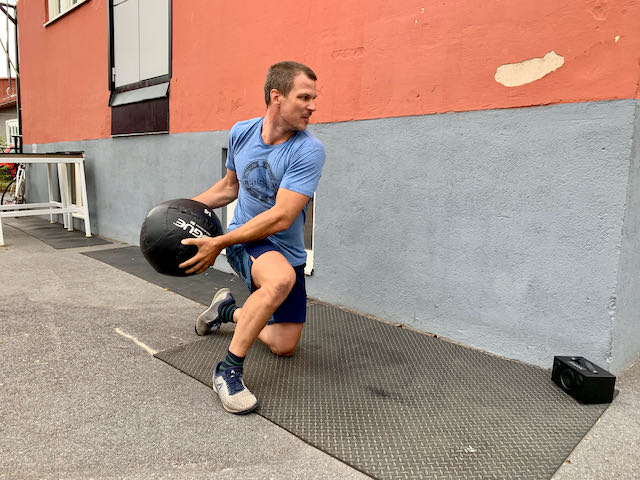
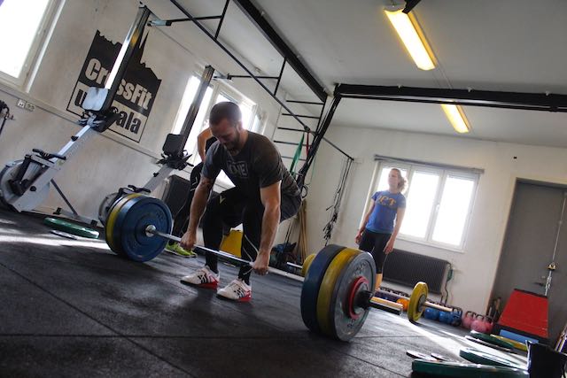
What separates successful athletes from merely athletes is the ability to execute fast and intense movements.
However, the attempt to forcefully perform a movement will create tension in muscles other than those needed for the movement, resisting the movement rather than supporting it. If you tell people to focus on engaging a muscle, it makes them think, which slows down movement. You can’t be thinking about your “traps”, “glutes” or “lats” when you need to move fast.
Relaxing helps to avoid giving force to the movement, instead letting the force come from the momentum of a turn of a foot or the hip, from a step or a stance, from the precision of the directness of the movement.
Moreover, relaxing is not only about the physical effort. It is also a matter of attitude, both in the moment and in the approach to training. Practicing and performing requires a quiet mind: a mind that is empty of expectations, ideas, and presuppositions. A mind that just does it.
How could one understand what it means to relax in a particular movement until one mastered that movement and, in a way, has become that movement, when at the same time mastery of the movement in itself involves already being relaxed. How can we teach and explain something that seems to require an experience of that thing in order to understand it?
It seems impossible to teach such subjective abilities through only direct instructions of how particular movements are performed. Rather it seems that coaching should be as much about showing the method of practicing, as giving direct instructions, and to instill faith in those methods.
This requires expertise, knowledge and facts, but also courage, empathy and understanding, and sometimes I think coaches spend a little too much time developing the first of these qualities, and a little too little time on the others.
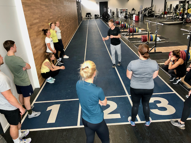
One of my favorite pastimes is watching coaches who balance all these qualities when they teach, watching them expertly swing in tune with a group of students and guide them to new learnings about themselves and others. Something similar to the conducted attunement of an orchestra, where there is harmony between different instruments that can both be recognized as part of the same melody, as well as distinctly different from each other.
Watching that makes me all warm inside.
I once got reprimanded by my seniors for saying in an opening speech for a course that I was about to teach that I was “a coach just like them, only possibly with more experience of teaching”, and that I invited open discussions that coming weekend, in order to create a better course.
This apparently, by my seniors standards, gave a bad impression of my organization. I was to be clear that I was to teach, to instruct, and the attendees would take in my knowledge. There had to be a clear hierarchy, for the pupils to take me as seriously.
I do not agree with them.
When it comes to parenthood, something that is often stressed is the importance of consistency with decisions and consequences. It is said to cause confusion when parents change their mind, and that this will harm the process of learning and hinder the conformation to the social sanctions that govern our practices.
Personally I think that what is really detrimental to this process of learning is when the parent does not change their mind when confronted by sound arguments.
The art of coaching is no different in this respect. Arguments are something to be taken seriously and compromises are often both possible and necessary.
As a coach or teacher, you can rely on the power you have by virtue of your office. It can be the right to distribute tasks, decide what is wrong or right, promote or demote, punish or reward. But there is also another type of power, a more informal one, which is based on being the one with the most experience or the greatest wisdom.
Submission is never the most developmental approach in any context or relationship. If you want to see commitment and development over time, there are many indications that it is wiser to lean more on the informal power than the formal one.
“The community stagnates without the impulse of the individual. The impulse dies away without the sympathy of the community.”
William James
In our time, there is often a call for strong leaders who are clear and know the art of simplification, but what we need is primarily something else: Leaders who stop managing, manipulating and making fools of their followers or pupils.
The coach, much like his pupil, must have an open mind to oppose his natural reaction to get stuck in rigid models that might not apply to this situation. He must resist his tendency to look for sets of rules, for an explanation, a formal notion or something else that does not capture all the complexity of a concept such as “learning”.
But all this is fine and dandy – yeah yeah – “as a coach you need to keep your eyes open, adapt to situations and try not to be Hitler”? Isn’t this just another way of saying “it depends”? And as with all arguments that advance to this, necessary but insufficient point we need now to proceed to what it actually depends upon, or what we can do to make better decisions here and now.
So I am going to make two practical suggestions on how further the chances to be that good coach, the one with the “open eyes”.
“Knowledge consists of knowing that a tomato is a fruit, and wisdom consists of not putting it in a fruit salad”
Miles Kington
1.Describe before explaining
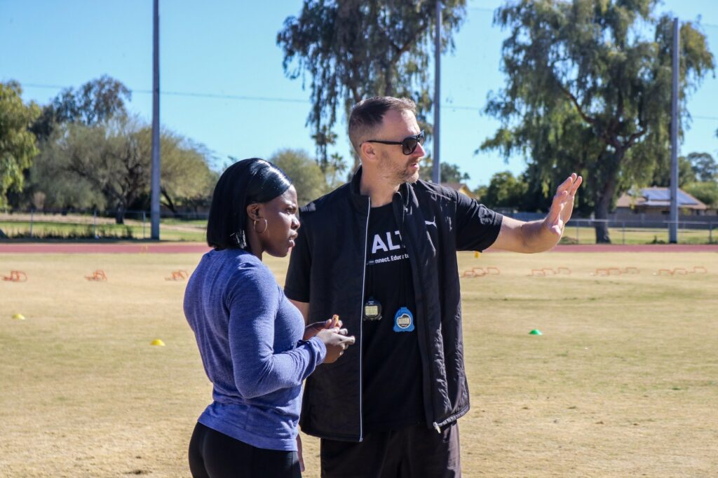
While athletes might be lacking in scientific knowledge, they tend to know a fair bit about their sports, and their practice of them. Discussions with them on these matters easily extend both into how to use the skills you have been working on in live action, and to sharpen the drills for improving them.
Ask the apparent questions in order to see what is already in front of your eyes: When do athletes struggle in racing or during competition?
At this point rid yourself of all the physiological models you have learned and describe those situations without explaining why they happen. That will momentarily rid you of preconceptions, and illuminate the path forward.
Use the language of the sport which is familiar to the athlete. You will move into a territory of training where your athletes have knowledge to add to yours. This will lead to relevant discussions on how to tweak the drills you will choose for them.
2. Learn a new skill
Us coaches do a lot of hard things like standing in front of a lot of people talking, directing and making decisions. But isn’t it often enough also the case that we no longer challenge ourselves with new skills while at the same time ask our athletes to do just that?
At this point in time we are often so far removed from learning new motor skills ourselves that we lose out on this aspect when we try to motivate people and encourage them when they learn such new skills that we ask them to do.
Perhaps we could be even better coaches if we would keep up to date with that feeling of how frustrating it is to be bad at something. How it is to damn well know how to do something, but still not be able to show it.
It is frustrating to fail. It requires finding positives in parts when the whole is a mess. Remembering this could be useful.
When asked for help or coaching we all too often show the final product, instead of meeting them where they are now. Instead of coming up with drills simple enough to provide a possibility for relaxation we show off.
Doing so can be more than a little demoralizing, and maybe we would recognize this better if we found ourselves on the other side of these situations regardless of how senior we are.
“A teacher who can show good, or indeed astounding results while he is teaching, is still not on that account a good teacher, for it may be that, while his pupils are under his immediate influence, he raises them to a level which is not natural to them, without developing their own capacities for work at this level, so that they immediately decline again once the teacher leaves the schoolroom.”
Ludwig Wittgenstein
Let’s take a practical example of bad coaching, where the coach specifically did not follow the advice above. The result was alienation of the athlete, with the risk of the athlete walking away from the challenge or even quit the sport.
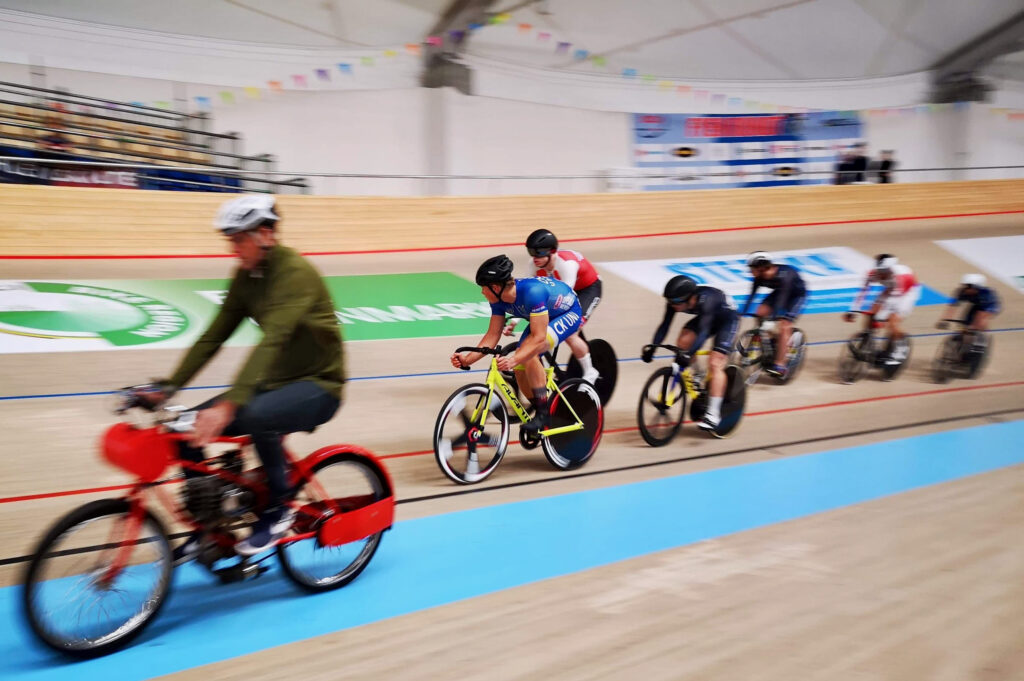
The sport of this particular athlete was cycling, and to give you some background I could tell you about the short summers and long winters in Sweden, meaning a large chunk of the yearly training has to be done indoors.
When cycling on a spinning bike or a bike steadily mounted in a machine to provide resistance, the riders only have to focus on producing power, whereas normally they also have to control the direction and stability.
One of my neighbors asked me if I could show him how to ride a bike on rollers, you know, the kind of rollers that you just set a regular bike on. The bike moves freely, meaning it could easily fall off the rollers if you make the wrong movements.
Cycling on rollers might provide less physiological overload, because of their larger demands for creating stability. Peak force and power output are lower than on an ergometer, but the need for balance while producing it makes this training quite similar to actual cycling. I have seen far more transfer of improvements to real cycling because of this.
The internet is littered with videos of failed attempts while riding rollers . This is not strange at all, because in the beginning it’s a little bit like trying to run on ice.
One has to be relaxed, but as we have noted one does not relax just because one is being told to do so. This video I found on random is a very reasonable first attempt.
Anyway, I filmed myself riding in my living room and sent the video “for inspiration”.
How do you think he felt when he watched this? How much could he value whatever large steps forward he took on his first sessions, when he put them relative to this rather than where he started from?
Experts in all fields appear fluid and natural but in reality they have made conscious efforts to shape the way they perform. Simply having the same knowledge of how to perform exercise is not what makes great coaches great.
“The philosophy of dissonant children”, https://www.researchgate.net/publication/230167370_The_philosophy_of_dissonant_children_Stanley_cavell’s_wittgensteinian_philosophical_therapies_as_an_educational_conversation
“On Heidegger on Education and Questioning”, https://www.researchgate.net/publication/311857931_On_Heidegger_on_Education_and_Questioning
“Quiet Minding and Investing in Loss”, https://www.academia.edu/43704333/Quiet_Minding_and_Investing_in_Loss_An_Essay_on_Chu_Hsi_Kierkegaard_and_Indirect_Pedagogy_in_Chinese_Martial_Arts
“Vi behöver en annan sorts ledare”, https://sverigesradio.se/avsnitt/att-vara-ledare-ar-inte-att-alltid-ha-ratt
“Only in failure, in the greatness of a catastrophe, can you know someone.”
E.M. Cioran
Picture some middle-aged dude with the habit of going down to the local wrestling club, always challenging the newcomers in the kids class to matches of greco-roman wrestling. He’s crushing them! Ripping them up! Throwing their little bodies in the air, slamming them back down on the floor, trash talking… He is 183-0 against them. He is the MAN.
Well, if Alexander Karelin, widely considered to be the greatest Greco-Roman wrestler of all time, would go down to the same club to wrestle the same kids he too would be 183-0 against those kids. If this was all that we had to go on to decide which is the better wrestler of our dude and the “The crane from Siberia”, apart from reverting into aesthetics, how would we ever know.
And how could our middle-aged friend ever truly know how good of a wrestler he is until he dares to challenge himself enough to fail, and therefore see where his limitations are?
Uncertainty is scary, but when you accept that uncertainty of things, the flip-side of that is that now you can go anywhere. If you accept the dangers of the Savanna, for example, you don’t have to stay crammed inside of that armored car on the road watching things from a distance.
But just like any experience that is quite special, it comes with a cost. And the cost of this type of existence is anxiety, dread, and all the rest of the feelings that come with plunging into the unknown.
For some to seek out, and stay, at these borders of what is comfortable comes completely natural.
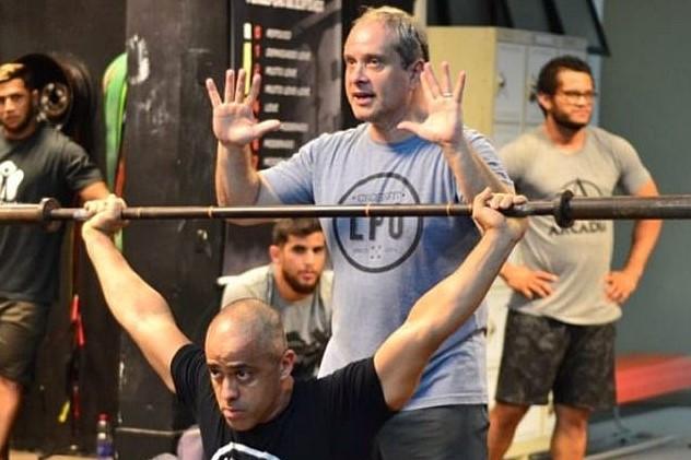
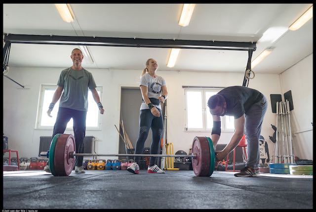
For instance I remember meeting Dragos Stanica for the first and unfortunately only time in my life when I was teaching a Course for Eleiko in Brazil a few years back, while the Brazilian nationals in olympic weightlifting was held at the same venue.
Dragos, a former weightlifter, who represented Romania in the 1988 Games in Seoul, South Korea, now lives on the outskirts of Rio de Janeiro from where he has his base, serving as the national coach for Brazilian weightlifting.
One of the nights, after the final day of competition, me and my colleague got Dragos by our table and when we got him started talking we never wanted it to end. That man had so many great stories from his life to tell, and it seemed all we had to do to enjoy them was to keep getting him (and us) beer.
He told us about his life, from his upbringing in a poor Romania, how he got to be a successful weightlifter, got recruited by a circus traveling the world, to stories on how he became the physical trainer for most of the Brazilian UFC superstars, and it just kept going, all the way into how he now lived permanently in a Brazilian favela, helping kids to learn to overcome their environment with his little weightlifting club as his teaching tool.
Of all the stories he told, the one I most often think back upon is the story of him starting weightlifting. He was 13 years old when he first ventured into a weightlifting club located in a basement.
“The lightest barbell they had was permanently loaded with 50 kilos, and I barely weighed more than that”, he said, “they showed me other lifters snatching it, and I wanted to do the same, but I failed miserably of course”.
He went on to give a picturesque description of how he came back, week after week, month after month, always failing to snatch the barbell from the floor over his head. It all seemed completely futile of course, but it became an obsession to him.
“And then one day I snatched it. I was very surprised” and he took another sip of the Brazilian beer, looking as happy as he must have been in that basement on that day so many years ago.
”If to describe a misery were as easy to live through it!”
E.M. Cioran
But most people are not like Dragos, not even if they are elite athletes. Faced with the possibility of failure, many might rather walk away from the challenge completely if not helped by someone to stand firm in a sudden storm of emotions.
For infants, all signals from the body or the world around them are causes of panic and result in screaming because they have not yet learned to put them into words.
With the help of its surroundings, it then trains itself to interpret both it and itself, and many things are then no longer perceived as threatening. This allows the child to move on and make wiser decisions. The screams are exchanged for productive responses.
But that presupposes that it has not been trained to shout when it is just hungry or experiencing something else normal.
That, in turn, requires the help of responsible adults.
Anxiety is an integral part of performing in sport for a majority of athletes, regardless of what level they perform. Being able to manage that anxiety can really help to produce a better performance. Under pressure, some athletes can produce a “peak performance” where they actually perform better, but the risk to be overcome with nerves is also always present.
This, in my mind, is one of the most important tasks of the coach: to help and guide their athletes to dare to challenge themselves, to dare to stay in these uncertain situations despite the flush of emotions that may overcome them. This is hardly done by pretending that those emotions aren’t real.
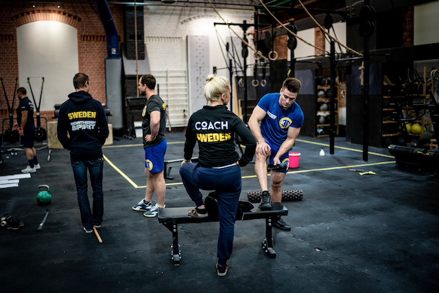
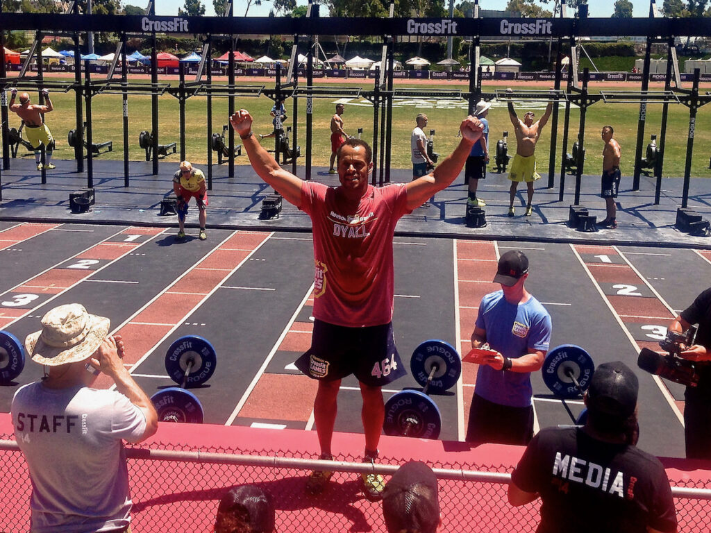
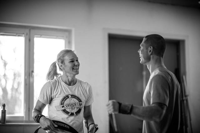
Many times I have seen trainers reassure their athletes when affirmation more likely was what they needed from them. One situation comes to mind, in the warming-up area for the European Regionals of CrossFit in Madrid. I was there coaching team CrossFit Nordic in their pursuit to put them on the podium of the competition.
Arriving with the team to the warmup-up area to get ready for our first event, I saw this Swedish athlete who I knew, running and looking unhappy on one of the non-motorized treadmills. Knowing that the first individual event wasn’t until all of the team events finished up, I walked up to her and asked what she was doing there and where her coach was.
“I don’t think I can compete in the next event, I don’t think I am good enough” was her reply, and you could see in her eyes that she felt both scared and lonely.
After some time her trainer appeared, and I overheard his answers to her expressing her doubts of herself as “Come on, you’re great, you’ll do fine, stay strong!” and I watched her try to smile and to look strong.
This athlete quit individual competition after this Regionals, which was the athletes first.
Maybe this would not have happened if the coach, instead of trying to sweep the feelings of doubt under the rug, would have affirmed those feelings, helped to put some words on them, asked if she has felt like this before, if so what she did, and how that felt.
To tell her that it must be hard, but nevertheless normal to feel this way.
Anxiety is a state comprising both physical and psychological symptoms due to feeling apprehensive in relation to a perceived threat. Each individual may experience anxiety slightly differently and it also may differ from situation to situation. For example, one Olympic weightlifter I worked with couldn’t get themselves onto the platform without feeling like passing out, while many CrossFit athletes would be physically sick waiting in line for their heats, or cyclists frequently abandoning longer and tedious races, not because of tactical reasons, but overcome with feelings of doubt.
It is natural when experiencing anxiety to want to get rid of the feelings because they are unpleasant, therefore people can seek solutions to avoid feeling like that.
If the anxiety becomes extreme an athlete may even get to the point where the only way to not feel like that is to stop competing or even quit the sport. This is a solution, as it might put a stop to these strong unwanted feelings, but the athlete might by doing so lose what’s most important to them (their sport).
A better option would be to accept anxiety, embrace it and learn ways of living with it.
Using only reason and empiricism to do this will for some always fail, for these methods can not explain reality with certainty. Then, to be able to cope with this uncertainty, one must accept that the aversions causing these feelings are real and that they are felt in this way, rational or not.
Letting them be real, then look around to see the things, in the same situation, that are experienced as positive. While some things are outside of our control, uncertain and in many ways terrifying, some things are always not.
Continually doing so the floods of emotions experienced in these situations will be decreasing with time. The wolves that hunted you become dogs, in time they might even bring you your slippers.
– But I believe what you are experiencing is a feeling. – It’s a horrible feeling. – I can see it’s unpleasant. – But like all feelings, it will surely pass.
From the movie “The Party” (2017), Directed by Sally Potter
This should not only be in the competitive setting. It has to start in the training hall, where one should not “win all workouts”. I am a huge believer in not pursuing perfection, for perfection is impossible to catch.
I have in previous posts argued that long periods of basic training has drawbacks when it comes to effectiveness and planning, producing unwanted adaptations, such as significant decreases in power and speed abilities, and taking up a lot of the training time available.
But these are not the only pitfalls of excessive periods of basic training.
First, the high intensity movements used in competition give the body fewer options to cope than using pre-tensioning strategies available through the stiffness of the muscles tendons. The lower intensity of basic training allows for, and it usually is done to strengthen the muscles contractile tissue.
But with less demands on the tendons, we risk that they become inefficient and come game time, when the luxury of inefficiency is not available leading to injuries (which put a stop to everything).
Second, getting back to my main point: if training looks too much like competition it becomes unbearable, or at least it does not provide enough variation to provide the means for improvements. But on the flipside, if it looks too little like competition it has no way of helping the athlete to cope, “learning the language of”, the uncertainty of competition.
Instead of more is more-approaches, where more necessarily means further from the demands found in competition, I once again propose a differentnot more-strategy.
Continuously challenging the individual participant by progressively increasing task difficulty during practice enhances motor learning and optimizes performance, while also helping the athlete to safely develop strategies to counter the frustration of being exposed to the slight possibility of failing.
“Failing to plan, is planning to fail”, and while this is good advice, as a coach you need to remember that the experience on the competition floor often is a very different experience despite all the training that precedes it, which often gives rise to emotions not able to plan for.
The way of being a better coach then turns out to be pretty similar in the training hall and on the field of competition: to take one’s nose out of the plan and look at the situation at hand.
See possible improvements for each athlete and manipulate exercise in order for these improvements to arise.
Do not reassure. This discounts the athlete’s fears, makes him doubt himself even more and reinforces the anxious behavior that got your attention. Avoid acting on your first impulse to counter them by reason. Instead: listen and confirm that feelings of anxiety, fear, doubt are normal.
Do not say what an athlete should not do or cannot do (Such a list would be virtually endless and quite useless). Focus on communicating what he or she can or should do.
Experts in all fields appear fluid and natural but in reality they have made conscious efforts to shape the way they perform. Simply having the same knowledge of how to perform exercise is not what makes great coaches great.
If so many people know how to do a barbell clean and the basics of how to coach it, why are some so good at developing lifters and others are not?
Science is great for predicting the average response in a certain situation, and while this is a good starting point that is all it is. The great coach also realizes that they are working with humans, with all the unpredictability and erratic behavior that might follow from that.
“The definition of insanity is doing the same thing over and over again and expecting a different result”
Because Einstein said it, it’s got to be true?
Well, first of all there is no substantive evidence that Einstein wrote or spoke the statement above. The linkage to the genius whose hair was always uncombed, clothing always disheveled, and who never wore socks occurred long after his death. It is one of many completely unsupported quotes attributed to him.
When one looks for the very influential statements’ real origins it seems like it originated in one of the twelve-step communities. Twelve-step programs are mutual aid organizations for the purpose of recovery from substance addictions, behavioral addictions and compulsions. Being communities who greatly value anonymity adds to the difficulty to identify a specific author to the saying.
Regardless of who first said what, the idea that one can try something and instantly see if it resulted in anything useful or not, is something that we mostly take for granted. From this we, usually without thinking much about it, similarly take for granted that if something did produce positive effects it would do so again if we kept doing it.
When doing so we fail to see that not all change and not all strains within a system are visible on it’s outside or by the parameters we measure it by.
Further it can make us rush on to try new things too soon. To give up when we would need to be patient and let the things we do bring about the change they could, given some time.
Systems can be analyzed in terms of the changes of their states over time. A state is an attempt to characterize, or define, a system by a certain set of variables. When a system changes its state its variables also change as a response to its environment and a completely different behavior might emerge.
This change is called linear if it is directly proportional to time, the system’s current state, or changes in the environment. They are called nonlinear if it is not proportional to either of them. In a nonlinear system very small changes might sometimes give rise to great changes of the system, and vice-versa.
Complex systems are typically non-linear, changing at different rates depending on their states and their environment. They have stable states, called attractor states. These are states that are preferred, and govern system behavior to stay the same even if perturbed. They could also be unstable, at which the systems can be disrupted by a small perturbation.
Examples of complex systems are the ecosystem, the weather, forests, organisms, the human brain, infrastructure, social and economic organizations (like cities) and ultimately the entire universe.
When these attractors are in such unstable states, exposure to what might look like the same environment, or such tiny changes of it that they can hardly be seen, could quickly completely change the entire systems behavior.
This type of change, which characterizes much of nature, is often abrupt and discontinuous. Systems experience periods of turbulence as attractors destabilize and create the potential for phase transitions (sometimes called bifurcations or tipping points). During these transitions, systems reorganize into new patterns of functioning.
A familiar example is the transition from liquid water into gas when boiling water. Under gradually increasing heat, the water remains liquid until the tipping point of 100°C is met and the sudden transition toward the gaseous phase takes place.
If one wanted to boil water but gave up when nothing happened after a minute or two, one would be prematurely looking for other ways to get things cooking.
Samuel Beckett, winner of the Nobel Prize in Literature, and most famous for his play Waiting for Godot. A play that was famously described by Irish critic Vivian Mercier as in which “nothing happens, twice”.
Two dysfunctional men encounter others along the road as they wait forever and in vain for the arrival of someone named Godot. They fill their idle hours with a series of mundane acts and trivial conversations as the world of the play operates on nothingness.
Surely the author of such a play could offer a counterpoint to the dominating “definition of insanity”? Something more useful to handle the everyday struggle of nothingness without prematurely abandoning or giving up on one’s efforts?
Sure enough, In 1983 Beckett offered a different perspective in his work Worstward Ho:
“All of old. Nothing else ever. Ever tried. Ever failed. No matter. Try again. Fail again. Fail better.”
What Beckett is telling us is that no matter how good the attempt, all actions inevitably fail to be perfect, then one must make another attempt and another, and the effort is in the attempt – not in the product.
In a non-linear world one could be considered mad if one would think that doing the same thing over and over again could not produce a different result. For both the person and the environment where the action is carried out is always different, if only so subtly.
Possibly the hardest thing to do as a trainer is to back off. To realize that while you are very important in some parts of the process of learning, most of the time must be spent simply doing.
I have a friend who is a very accomplished trainer, and who have few superiors when it comes to designing exercises. His skillful eyes see not only unsatisfactory movement outcomes, but also at what point initial flaws that might be causing them arose. On top of that he has great understanding for manipulation of the exercise to open up for better movement patterns, as well as being skilled in communication.
We often teach together and his imagination and sharp eyes never seize to impress me. Then things go wrong. He’ll have the athlete do the exercise a few times, or maybe a week, watching closely. If he sees better outcomes, he goes on to take on the next pattern to be sharpened.
Change takes time.
Much like parents often end up trying to fulfill their dreams through their children, teachers often get too involved in the process. Over-coaching and pushing too quickly can be just detrimental to the development of new and efficient attractor states as the opposite.
In other words, it simply happens. The coach, the midwife of all those new skills, is simply momentarily assisting in the process, but not making it happen.
Practicing and performing require a quiet mind: a mind that is empty of expectations, ideas, and presuppositions, that is open to what happens in the presence of every aspect of a movement.
To be a masters trainer, on top of all your technical wisdom, you need to be patient.
To see possible improvements and manipulate exercise in order for these improvements to arise.
To communicate so that the student understands what constitutes a good rep versus a less good rep.
Stepping away and letting the student find his or her way of increasing the frequency of good reps, until it is something done without thinking. The failed reps in the process is what eventually lets the good reps just happen. (very hard, and often forgotten)
Staying cool and detached yet a little bit longer, remembering that just because some good reps are being done, it does not mean that they just happen, just yet. (requires the patience worthy of Buddha himself)
Coaches momentarily assisting the process I said… But sometimes that moment is long. One week? Four weeks? Months?
It is impossible to tell how long it takes for a new attractor state to emerge, but in my experience it varies not only between individuals, but also with time for the same person. All we have is to stay rooted in the present and to evaluate the fluctuations of the athletes results.
When an attractor is getting more stable there will be less fluctuations in performance. In order to see this we cannot vary the exercises and workouts too much.
A master coach who did take this to great lengths was Anatoliy Bondarchuk. A former Olympian himself, he turned to coaching after his career and is widely regarded as the most accomplished hammer throws coach of all times. He developed what can best be described as completely response-based programs. His method largely consisted of repeating the same session over and over again, with no wave loading of training variables and abilities, and no changes in strategic or qualitative elements.
Will there be no variance in such a system? Surely there will be, for in a complex world both the person and the environment is always slightly different.
Plotting the response to similar sessions or exercises over time one can clearly see the phase transitions of our athletes.
A program with little variation allows you to see the states of the system over time. When data and form seems stable, then we can also assume that the attractor states are stable. When this happens, but not before, we should be increasing task difficulty in order to force adaptations via yet more phase changes.
One note of warning though – one might be tempted to think that we now know how this athlete responds to training, and would be able to predict the time to adaptation or phase transitions for the athlete. But when a system changes its state, a different behavior will have emerged.
While we now know our process of exercise selection and communication likely functions well for this athlete, we can’t ever relax and be the lazy coach.
“For the young the days go fast and the years go slow; for the old the days go slow and the years go fast.”
Anna Quindlen
Regardless of what specific method one adheres to, for there are many possibly great ones, one thing I see more from the experienced coaches is that they are likely to let things take their time and by doing so allowing for more possible growth of their athletes.
In the first article of this series I explored the risks of assuming that there is something fundamental beneath the surface, which must first be optimized in order to increase performance later on. In the second article I challenged the need to continually increase physical training load, suggesting to focus instead on adaptation of task difficulty to where our athletes are exactly now.
In this last article of the series we will continue to explore methods to stay in the present, and how the use of our language can help but also overthrow our attention to what is really going on and hinder the transfer of the exercises we prescribe.
As we have seen, the promise of the ideal is repeated over and over again but never fulfilled. When technology was invented to measure oxygen consumption, blood lactate concentrations and force it gave rise to new models for training. Now the recent ability to sequence DNA is looking to change the way we measure and prescribe training.
While this way of looking at the internal processes of the body certainly has merits to many sciences, it is still not able to add much to the decision process constructing training programs. Just like with the preceding reductionist approaches comes the same possible pitfalls.
We could also measure the length of fascicles, concentrations or flux of chemicals, energy storage or the efficiency of the electron transport chain and… Well, it’s likely to be a mess to bring all those parts together in a general capacity. The whole is not the sum of its parts, despite how magnified they may be.
The aspects of things that are most important to us are hidden not because of their depth, but because of their simplicity and familiarity.
The philosopher Ludwig Wittgenstein once described the situation as it is as if a man is standing in a room facing a wall on which are painted a number of dummy doors. Wanting to get out, he would fumblingly try to open them, vainly trying them all, one after the other, over and over again. But, of course, it is quite useless. All the time, although he doesn’t realize it, there is a real door in the wall behind his back, and all he has to do is to turn around and open it.
Having explanatory models of how it all works, seems to be helping us to take the right actions. But the problem with the concept creation is that it assumes that by creating concepts, we can lay down in advance what it is we are thinking about. In plain English, there is really not much evidence supporting the theoretical concepts of phase potentiation, but we have a hard time to see this since it is all we know.
To help our man get out of the room all we have to do is make him look in a different direction. To do this we should turn things around, away from the safety of dogma, and look at what is hidden in plain sight.When do our athletes struggle in racing or during competition? Describe those situations without explaining why they happen.
This brings us to the topic of terminology, on how to best communicate with the people we coach.
Concept language is used to describe words or constructs that bundle a lot of actions and interactions under a simple word. To transmit less detail and more fundamental aspects of information faster and easier, mainly by experts of a defined field.
Complementary training, meaning all training carried out away from the field of the game, with the intention of helping successful execution of skills in the game itself (or a more functional life for that matter).
Coaches, specifically us who provide help with complementary training, are usually using the concept language of our field, as opposed to the language of the game itself. We use constructs that are natural in the gym, like “strength”, “strength endurance” and “speed”. We speak a language of “intensity”, “volume”, “sets” and “reps” with the athletes that we train.
When athletes are new to complementary training they usually struggle. They have a hard time to understand our lingo and to perform the training we prescribe with it. When we invite athletes into this world, filled with new mysteries to solve, they will eventually get better and better at speaking our language and doing our type of training.
But this was never the end goal.
It is not enough to show how clever we are by showing how obscure everything is
J.L. Austin
There is some evidence that memories are stored in the same brain regions as they are perceived. This means that not only what you mean when you phrase your coaching cues matter, but also how the athlete interprets them and in what context the training is carried out for their subsequent retrieval.
The way language seems to provide a gateway into athletes’ motor cortex is quite stunning. Studies show that when participants hear verbs like lick, pick and kick it activates the respective brain regions of the tongue, arms or legs.
By using language so different from the field of play, we might accidentally be creating a rift between the athletes training and the application of it. By using ourconcepts instead of mapping into the common language that is better understood by our trainees we are limiting the transferability of the training they do .
Sports is a practical matter. It is not about words, but rather about actions. Action language, on the contrary from concept language, is the language used to describe only relevant details in a clear, concise and objective way, transferring details without judgement, often with a more direct purpose. It tells what to do in a specific situation of a game.
When we start with what we see, rather than from physiological constructs, we are more likely to be able to create terminology that ties the action language of the sport and concepts of exercise science together. Then we can utilize this terminology in a coaching process that is individualized without becoming abstract.
The athletes will perform their exercises more purposeful and they will intuitively know how to use the skills they are strengthening. And, although they might not be well versed in your world, they often are very knowledgeable of their sport. They know themselves and they will be able to help improve those exercises in a constructive way.
In this the third series we will show how one could implement the proposed methods by using cycling sprinters as the example.
A muscle fiber generates tension through cross-bridges of actin and myosin. Under tension, the muscle can be made to lengthen, shorten, or remain the same. Muscles also have elastic properties where energy can be stored to increase force, but only for a very short time. When a muscle is not tense it is “slack”. To produce movement, that slack has to be removed by pretensioning.
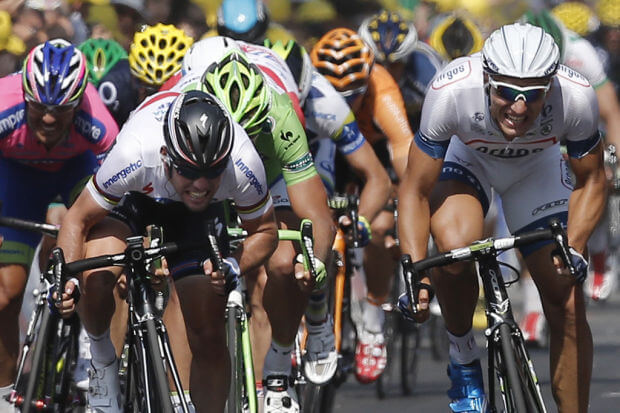
At high speed and high power the demands for contraction velocity, pretensioning and efficiency of storage, and return of energy are greatly increased. As a result there is little positive transfer between different types of muscle contraction. In cycling most muscle actions are shortening contractions.
Cyclists produce higher peak pedal power and rate of force development on a stable cycle, commonly referenced to as an ergometer (like a watt bike, a spinning bike or a trainer) than when riding in a velodrome.
When sprinting on the ergometer, the riders only have to focus on producing maximum power, whereas on a bicycle they also have to control the direction and stability whilst trying to produce maximal power. Also, one of the biggest factor to overcome during cycling in aerodynamic drag which is not easily simulated in a gym.
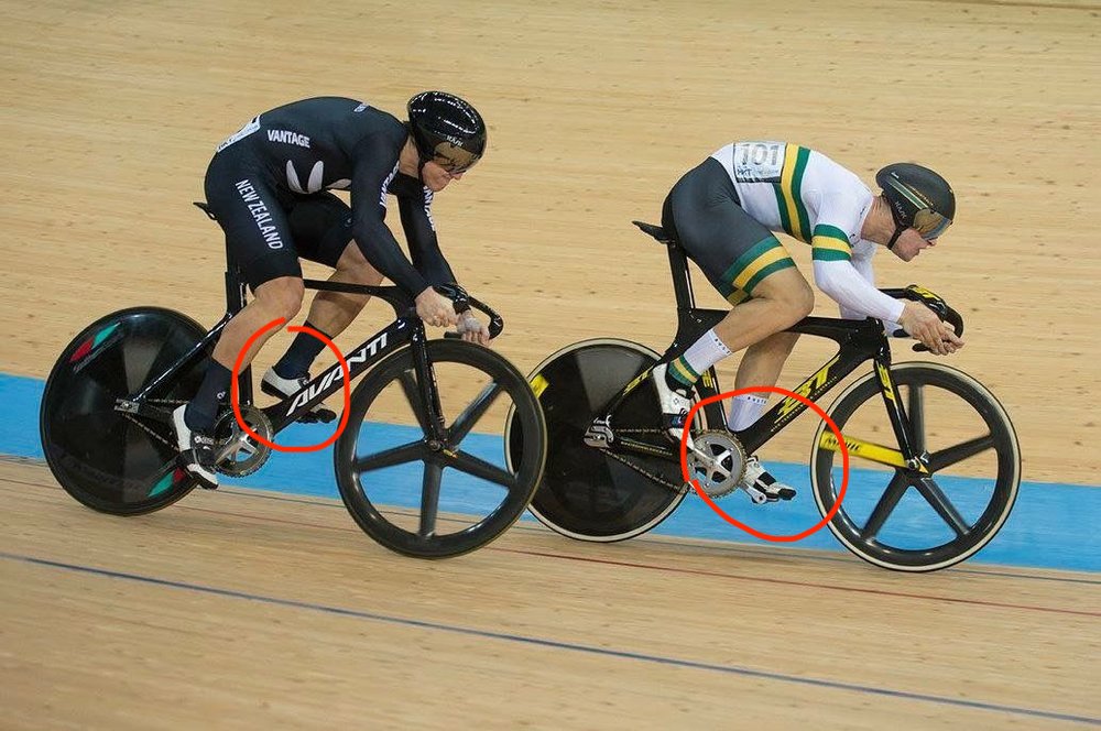
Because of different demands there is an altered riding position observable as difference in hip, knee and ankle angles.
With the principle of specificity in mind there would seem to be arguments for the the track cyclist to train on the track, or to find other ways to challenge stability if that is not possible.
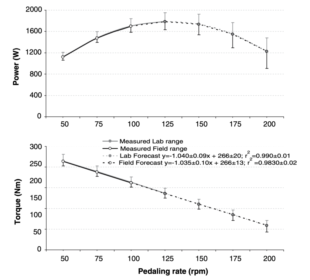
Torque-pedaling rate and power-pedaling rate relationships for laboratory and field tests, estimating “optimal cadence” in Elite track sprint cyclists (Gardner et al, 2005)
Cadence, or pedaling rate, is an important factor influencing the economy of motion, power output and the development of fatigue during cycling. In track sprinting the use of fixed gearing makes this a very important consideration at race day, but also to guide training. The inability to select the best gear for specific situations during a race, forces a decision on which gear would be overall most suitable for a rider in all situations. Some factors influencing this are the type of race, the opponent and the rider himself.
Bigger gears give the opportunity for higher maximum speed with less fatigue. If one is able to get up to speed and then to effectively spin it around, that is. With higher inertia comes higher demands of force.
There has been considerable research in what is called optimal cadence, the cadence where peak power is achieved. Given the importance of contraction velocity and efficiency in high speed and high power movement it is thought to provide important insight in the selection of pedaling rate, and therefore appropriate gearing.
Optimal cadence is highly correlated with the amount of fast-twitch muscle fibers, and in a sport where the ability to push bigger gears are so rewarded as it is in track cycling, there is likely not much drawback in continually training to increase their proportion. Given the low risk of gaining mass when doing large volumes of training, there is little reason for the road sprint cyclist to think differently.
As with other constructs there is a catch to letting peak power testing dictate training decisions. Those tests are almost always carried out with very little pre fatigue and from a stand still or low cadence. Following periods of exertion cadence at peak power has been shown to change. Higher velocity provides less time for cross bridges to form, and therefore the demands for the speed of contraction increases. The demands of the athlete shift with each situation and each athlete.
You can’t make an omelette without breaking some eggs…?
In a small country like Sweden, with a limited talent pool even in our national sports (football, ice hockey, skiing), we need to adapt our coaching to improve each person in front of us, rather than the other way around.
One would need to look at the specific situations each athlete struggles with to best construct exercises to increase their capacity in those situations.
Sven Westergren is the current Master national champion in Match sprinting. Match sprinting is the discipline where two opponents go head to head for 3 laps, or 750 meters. He is big and strong and able to push bigger gears than his smaller opponents. They however have the upper hand when it comes to quick bursts of acceleration from lower speed.
Tactics comes down to controlling the pace. If Sven is able to keep the base speed high enough to prevent aggressive “jumps” from his opponents they tire quickly, and have little to do when he eventually accelerates to top speed. In order to strengthen his ability to do so, exercises for acceleration and maximum speed can be constructed to involve a build-up beforehand.
With little access to the only Velodrome in Sweden, which is located more than 2 hours drive from where we live, and knowing that the transfer of skill development from ergometers to the track might be low, we do most of our training during winter season on resisted rollers. This is not ideal, but better than other options.
Rollers might provide less physiological overload, because their larger demands for creating stability. Peak force and power are lower than on an ergometer, but quite similar to the track, and we have seen more transfer of improvements on to the track because of this.
We should use our coaches’ eyes when we construct exercises for our athletes, but if we can formulate them with language well understood by our athletes, we are improving both their transferability and the chance for better feedback. A clear goal for our exercises also allows for better judging if the exercise was successfully executed and functional.
A possible way to create a helpful terminology would be to first define a game model based on the broad actions taken in their sport.
For track cyclists we could construct such a model by going through each broad component carried out in a race. A very simple example would be to specify the possible actions to master as the start, the acceleration, maximal speed and speed endurance.
For each of these areas we can assign suitable actions, which would be a good starting point in order to create a more individual and usable “dialect” of a general sports language. Actions however do take place within the boundaries of space and time. If we sat down in a car and all everything that was told to us was to “drive” the action would seem less connected to its environment than if we were also given instructions on how fast and in which direction.
Similarly our cues will also benefit from the inclusion of direction and distance.
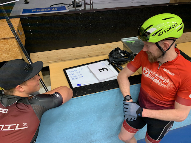
Christoffer Eriksson is the Nordic Champion in Keirin. Keirin is an event similar to the match sprint but features between three and seven riders competing in a sprint race of 3 laps after having followed in the slipstream of a pacing motorbike for 3 laps. The motorbike gradually increases in speed before peeling off and letting the sprinters battle it out. The event is fierce, fast and unpredictable, with many split-second decisions about when to hold and when to attack that have to be made under fatigue.
Christoffer has lower top speed than many of his opponents, but on the flipside he is perceptive and he does not tire easily. In competition he cannot just muscle himself to wins but instead has to see how the match unfolds. He wins by finding the opportunity to get a gap early, or to follow the strongest riders when they do so. Using his strength to not get boxed in, and accelerate to fill gaps is an important quality for him.
One exercise to practice this ability could be to build, then simulate staying on a wheel, relaxing to get some distance in order to use the slipstream to get enough speed to go past on the outside. We could call this exercise “hit, fly, hit”.
In order to build the language for this we should consider the actions involved in it. Most important is the verb that should be the main descriptions of the action to take. I’ve often used the word “push”, as it is pushing the pedal away we would like the athlete to do. But considering that pushing is something that could be done slow I prefer “punch”, which I think would be a perfectly fine option. You can push slowly, but you can’t imagine punching slowly.
Knowing about the very specific encoding of memory storage, I would like to use a word less associated with the upper body. I would propose using “stomp”, which would seem as a similar action as punching, but for the lower body, where power is most important for cycling.
When describing the exercise, I would use something like “Build up to speed and and then stomp as hard as you can to go faster, closing the distance to a breakaway rider. Then stay as smooth and effortless but without losing cadence, and then again stomp hard to accelerate past”.
In order to sharpen the action cue I prefer to shorten it to a minimum. Keep the action, direction and distance, and end up with “stomp fast forward”, and after the “fly part” again tell Christoffer to “stomp hard past”.
The exercise will be tied to race tactics, and we would be able to get a nice feedback loop going in order to improve future exercise according to the needs and skill level of the rider.
The skeptic could point out that the examples given in this series of articles appear to be quite simple. That all I do is to observe my athletes, and when I think I’ve seen what needs to be improved upon, I have them do that very thing. Yes, with some variation, and sure, carefully considering communication and possible improvements of the exercises – it all appears to be so simple.
They would certainly be right. Even though I would argue that doing the simple thing well, is not easy. Let’s also describe how one could use the same methods to develop something less like what is performed in the sport itself.
When an exercise is very specific, by definition it has a low degree of overload. If we would like to lift the middle of a rug from the floor, we would do best to direct most of our lifting to that point exactly. If we want to maximize how high we could get it, we would also benefit from at the same time lifting at the edges.
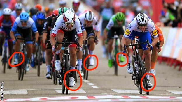
In elite sports, you rarely win with the distance of a landslide. More often with the small margins visible in the loser’s sigh. The athlete also needs the marginal gains found in general overload.
You have to appreciate the impact that variation and change has on how an athlete reacts to training across the board
Derek Evely
The upper body is involved at a remarkable extent when cycling hard compared to when cycling less hard. The degree of negative relation between upper body asymmetry and maximum cycling power production is quite exceptional.
This should not come as a surprise – in high intensity movement the opposing forces are so great that muscle fibers have to stay close to their optimum length, and as the feet are attached to the pedals, there is less flexibility of positions in the lower body. One can imagine how much this must challenge the trunk and the pelvis when force is applied into the pedals. Studies also indicate that compromised coordinative patterns for the ankle joint correlates with loss of power.
For the cyclist who wishes to win in a sprint this would seem to make an argument for
Upper body training (Pullups and Dips?)
Hip strengthening (Hip thrusts seem to be popular)
Core training (oh, those circuits that burn so good)
Ankle strengthening (Calf Raises, for more of that sweet burning sensation!).
While there is nothing wrong with these exercises, I would treat such isolation as things we do at the end of the session, after we’ve done everything else.
In movement, force produced by muscles moves through the body. Patterns between muscles occur with the changing demands of force in order to develop synergies. The whole body efficiently forms a unit capable of more force production than any of its muscles in isolation.
Again, with the principle of specificity in mind, there seems to be an argument for multi-joint compound movements in the gym to maximize transferability of increases of strength.
The need for variation is fulfilled already if we make sure that there is a large extent of overload.
“The human race shouldn’t have all its eggs in one basket, or on one planet. Let’s hope we can avoid dropping the basket until we have spread the load.”
Stephen Hawking
In bicycle sprinting you need to subdue very heavy resistance, especially in starts and acceleration. Further, these efforts must not make you so tired that you can continue to turn around those heavy gears the distance required to complete the race. Being strong for the sprinter is very specific.
In some of its disciplines, like in the match sprint and Keirin, a modernization of tactics has raised the need for top speed over acceleration. This has forced the riders into an arms race for the capacity to push bigger and bigger gears.
In earlier posts we have explored the balance between specificity and overload in the gym setting, and isolated the following basic rules
Keep movement somewhat similar in movement patterns and stimuli
Overload as much as possible while satisfying rule #1. Large load means larger neural adaptation and higher percentage of muscle fibers being recruited.
Anddo not let the main movement mechanics break down or change during the set
I argued for single leg movements for developing maximal leg strength for sports played on one leg (cycling, team sports, track and field, racket sports, etc) and double leg movements for those that have movements performed symmetrically (powerlifting, weightlifting, CrossFit, etc).
Possibly we could tweak this even further.
Before we go on to explore this I’d like to point out that I do not propose to exclude single joint general movement, despite having less obvious benefit. In fact I have all of my athletes do such movements, like pull-ups and dips, but they do it late in the session, after the more contextual work is done.
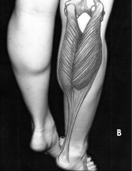
The way our muscles in the lower body are structured allows for a unique role in the transformation of rotation in the knee joint into the production of high force. Biarticular muscles are muscles that cross two joints rather than just one, such as the hamstrings which cross both the hip and the knee. Rectus Femoris in our quadriceps and gastrocnemius in our calves also have this property.
These bi-articular characteristics allow for extending the joints one by one in a sequence called the proximal-to-distal sequence more commonly referenced as triple extension. Extension of these joints one by one allows at least one of them to have a favorable translation relationship throughout the full extension.
This sequence allows for the possibility of more net force production, but in order to function properly the extensions should be completed in a certain order.
An ankle collapsing during the pedal push does not translate into movement of the pedal, but still cost energy. To prevent this leakage of force efficient cycling pedaling depends upon the ability to keep the ankle locked into position.
If the push downwards is done with a highly extended or flexed ankle the extension movement becomes rapidly less efficient. It would seem that cycling therefore cannot fully use the benefits of the triple extension.
During the sprint, ankle joint power decreases more rapidly than power at other lower limb joints, while hip extensors and knee flexors sustain their power for a longer time at higher rate.
The hip extensors are also the strongest muscle group in all velocities, followed by knee extensors and hip flexors. The weakest muscle group are the ankle flexors.
This seems to further support that there are differences in the efficiency of the pushing sequence with fast cycling, possibly at least partly as a result of not being able to execute the triple extension in the most efficient sequence.
Road cycling too involve recurrent demand for high force output, with little possibilities for perfect execution of the the proximal-to-distal sequence
New inventions in technology to measure performance in endurance training changes the way training is conducted and planned. The way things work in the strength world is no different. Traditionally the measurement was the weight on the bar, but lately bar speed, or power, has been popularized as a way to monitor performance.
More contextual always means less optimal for overload, meaning that athletes will always have lower numbers to show for their efforts. The systemized way of using such constructs could potentially bias us to high performance in these constructs, rather than to look for more contextual performance increases.
It will also subconsciously nudge us toward movements with the highest efficiency, regardless if we do not have these options for movement execution on the field. This is often defended with references to higher neural stimuli of these exercises. High effort in more contextual movements will also have equally high neural stimuli, despite lower measurements, as an effect of their lower mechanical efficiency.
Very seldom do we train strength in the gym with our joints in such non-optimal positions. Since muscles do change their optimal length and other properties with exposure, this is the whole point of strength training, and given that the coordination of chains of muscle is no less trainable – maybe we should?
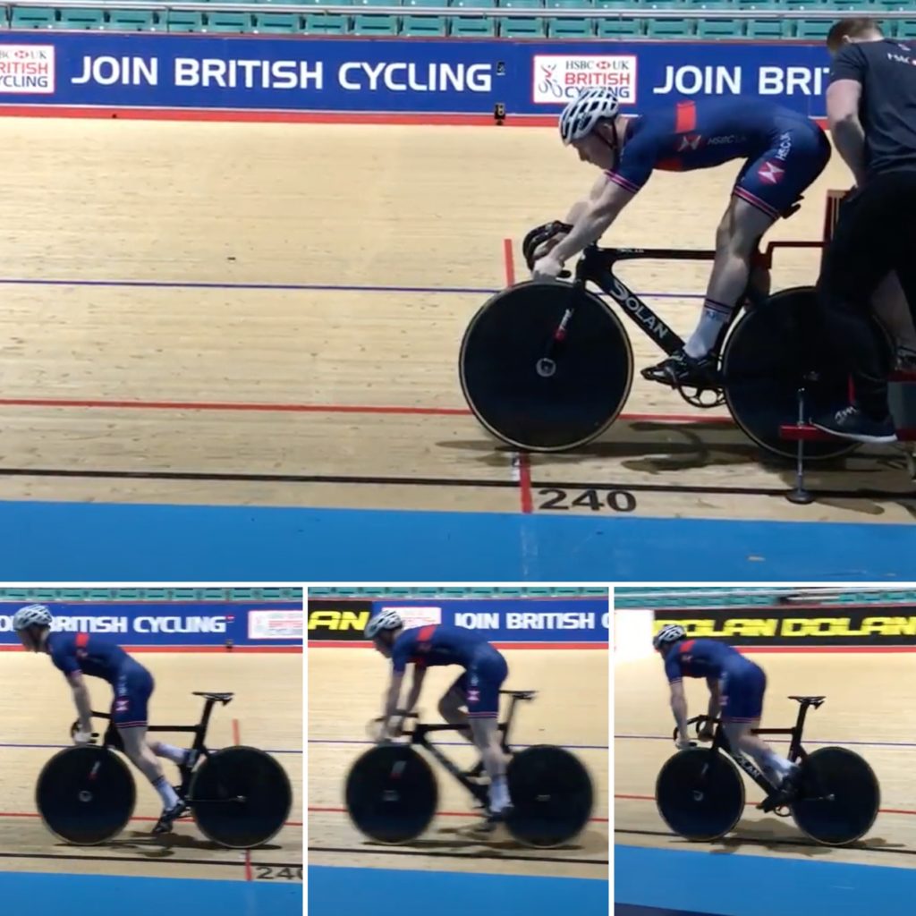
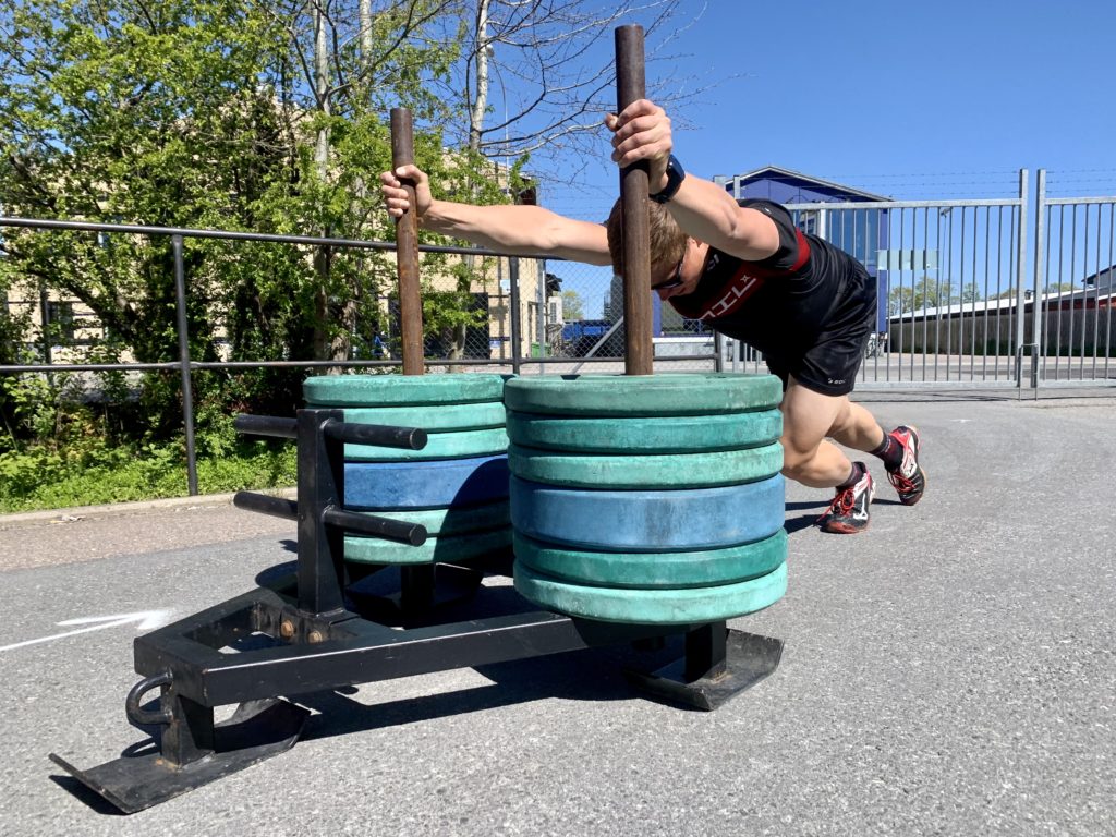
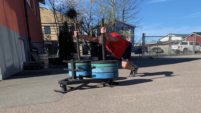
The standing start is no different from seated pedaling. If the knee joint and hip joint creates force by opening up, the ankle must stay fixated in order to translate this force from above into the pedal. If it does not there is a leakage of force.
As we found in an earlier article the split squat is a fine example of an exercise capable of generating a lot of force. Even more so with the added stability of the hands. We can see that the ability to transfer force through the ankle is one limiting factor in the video of the standing start above.
Possibly we could try to combine a dynamic high force output from the hips and the knee joints with a static high force demand of the ankle?
As cadence increases, the time we have to create force shorten.
Disregarding exactly what the optimal pedaling rate for high power sprinting is, it is definitely high enough to not allow for inefficiency. For us to develop efficiency to perform unloaded high intensity movements, we should practice pre-tensioning with the use of co-contracting muscles alone.
This could be done with high power ballistics movements, such as jumps, especially from static positions with the least possible help from pre-loading and counter movements. I see few drawbacks doing some of them from mechanically challenged positions similar to what you would find in bicycling.
The splinter in your eye is the best magnifying-glass.
Theodor W. Adorno
The main reason we still lean so much on these perfect systems of explanation for decision making is that they provide the false safety of the ideal. Numbers are clear and concise, actual situations are messy. But in that mess there is also information that is lost when quantified.
A magnifying glass quantifies and enlarges an image, but the spectator cannot truly construe meaning from what is magnified. Only when we get a “splinter in our eye” we are forced to stop to regard the things that do not fit in. The flaw in vision, becomes a way of seeing better.
To say something about particular situations risks exposing our ignorance. Our challenge then, becomes not to hide from our possible ignorance, but to embrace that risk.
In the realm of sports science what can be thought of as classical periodization was originally discussed by Russian scientist Leo Matveyev and further expanded upon by Stone and Bompa. Periodization is a logical method of organizing training into sequential phases and cyclical time periods in order to increase the potential for achieving specific performance goals. All while minimizing the potential for overtraining.
Phase Potentiation is the strategic sequencing of programming phases to increase the potential of subsequent phases and to increase long term adaptive potential. Theoretically, using this concept, peak performance occurs in a controlled way as the phases are stacked on top of each other.
When examining the success of classical periodization concepts they fail to convince of their superiority over more concurrent approaches to the planning of training.
Not only are these long detailed and rigid plans vulnerable to unplanned periods of non-training – what do we do when the athlete gets ill? – but also that we just miss our mark, either on the resources available for training, or the speed of progress we ended up with. As we are working under either of the two false assumptions that averaged group-based trends accurately reflect likely individual responses, or that the individual response can be extrapolated to work for a group – our plan will only provide a false sense of security.
These methods with long cycles of mostly general work are also quite time consuming. For most sports disciplines, the packed competition schedule makes it difficult for coaches to adopt them, as there is simply not enough time during the season to improve poor form.
However, the most important drawback is their very low rates of effectiveness. When scientists have looked at the amount of athletes who are achieving the season’s best result at the seasons most important events, like World championships and Olympic games, the results are disheartening. Seldom if ever more than 1/4th of the athletes manage to deliver their top results for that season.
The theoretical and speculative “delayed training effect” concept assumes that training basic capacities at earlier phases of the training plan has positive effects on actual performance long after they are taken out of the training programs, replaced by more sport specific exercises. They also produce unwanted adaptations, such as significant decreases in power and speed abilities. Coaches might ask themselves whether basic training is a real basis for competitive performance, or whether it is a loss of precious time to athletes.
To be fair, basic training is not only done for peak performance but also for the sake of injury prevention. There is also plenty of evidence suggesting that what is likely responsible for a large proportion of non-contact, soft-tissue injuries is not training load as such, but rather excessive and rapid increases of them.
It is likely that the positive adaptations in muscles and tendons provided by longer periods of basic training may also be obtained by typical strength and power exercises. Exercises which can be implemented with little to no negative effects during the course of the season.
The stakes of unsuccessful performance at key competitions are high, with evidence suggesting that more severe psychological consequences are a distinct possibility. Failure to meet performance expectations include anxiety, interpersonal hypersensitivity and coach-athlete relationships falling apart.
“Speed is the most precious thing in swimming. It is what it is all about. I do not understand why you would spend weeks and months not training speed, then hoping it will come back when you taper and race. I believe you must always be within one second of your personal best time at all times of the year. That you must train for speed all year round. That your sprinters must sprint often and race regularly throughout the year.”
Gennadi Touretski
In the 90s the “Speed through Endurance” philosophy that reigned supreme in Australian swimming was challenged by the Russian coach Gennadi Touretski. This “more is more” philosophy was to work hard to first develop an aerobic base for 10 to 16 weeks (or even longer!), then to significantly reduce training volume close to the competition. The idea was that the more you swim, the more efficient you become and the more efficient you are the faster you can swim.
Touretski, the coach of one of the sports all time greats, Alexander Popov, was recruited to rejuvenate Australian swimming after a poor Olympic result and he did so by removing the (imaginary) certainty of linear adaptations provided by a base training phase.
He warned to assume speed will return once it is lost, and was wise doing so. The “delayed training effect” is not completely supported either by science or practice and its use as a tool to improve actual results are very unpredictable. There is simply not much basis to sustain the idea that the body is ordered into basic and specific capacities and that the overloading of a given basic capacity will suddenly “supercompensate” later in the training cycle.
When you have a capacity, you can certainly lose it (and haven’t we all experienced that). But that risk is way lower than the hope for you to gain a completely new capacity at a later point in time. For that reason he included speed training at all times of the training program, throughout all of the year.
“I think coaches do too many drills. Drills do not improve technique. They teach the basic movements of the stroke. To improve technique you must work with the individual swimmer, over a range of speeds, from slow to race speed and give them constant feedback about their technique, talk to them about how it feels and help them to develop their own technique. Every swimmer is different – every technique is different.”
Gennadi Touretski
Instead of general drills he believed that technique is a personal thing, and that training prescription should not be about doing a lot of general drills. Rather it should be about optimizing the technical efficiency of the stroke of the individual swimmer. Start with what you see, and practice what you see is needed for that particular athlete.
He would walk with his swimmers continuously throughout the session, ask them to swim initially at a slow speed, then have them progressively increase speed until he would notice a technique inefficiency. He would then describe rather thanexplain what happened and then figure out a cue to address the inefficiency he had seen.
There is plenty of evidence to support that increasing the physical load of training in the form of exercise intensity, volume or duration can be successful in order to enhance training adaptations.
When looking for the optimal adaptation found at the upper limit of tolerance, we expose ourselves to very small safety-margins of error. The presence of deep uncertainties linked to working with human beings challenges decision making by questioning the robustness of all purportedly optimal solutions. Knowledge about historical adaptation yields little to no information about how our “optimal” solution performs if the future surprises us, and they do not guide us to solutions that might work well if the predicted future does not come to pass.
Physical load can only be increased so much, and often this “progressively do more, do harder”-philosophy eventually pushes athletes into injury. And regardless of the progress made before this, injuries put and end to all progress.
Traditional methods for decision making require agreement about the current and future conditions and only then to analyze our decision options.
In a paper published by the World Bank on developing new processes for decision making under deep uncertainty, the research group suggested that alternative methodologies can help in managing uncertainty. These methods start the other way around by stress-testing options under a wide range of plausible conditions. All without requiring us to agree on which conditions are more or less likely, and against a set of objectives.
In the context of sports performance the traditional methodology would be to construct a training plan by starting out estimating the future capacity, form and other factors. For example to predict how much a specific squat cycle would increase squat numbers, and how much that in turn would affect sport performance in specific numbers. Only after these predictions are made we would evaluate the possible upside and downside under these assumptions.
This is problematic on two levels. First, many important assumptions are buried in models, rather than in front of decision makers and therefore vulnerable to bias. Second, many factors are difficult, if not impossible, to predict and risk to cause a gridlock in the decision process.
As an alternative, we could identify the plan that is robust, working well across all the scenarios by “stress-testing” our options under a wide range of plausible conditions. All without requiring us to decide or agree upon which conditions are more or less likely.
This means to imagine different outcomes from many possible methods. Squat numbers increasing by 15kg, 10kg, 5kg, staying the same or even regressing. Which methods end up with the highest satisfaction and lowest regret under all possible outcomes, including high or low transfer to sport performance?
When faced with the possibility of multiple outcomes we will end up choosing “no-regret” or “low-regret” decisions. Decisions on reduced time horizons that have high utility no matter what the future brings. They will be more reversible and flexible, and have larger safety-margins.
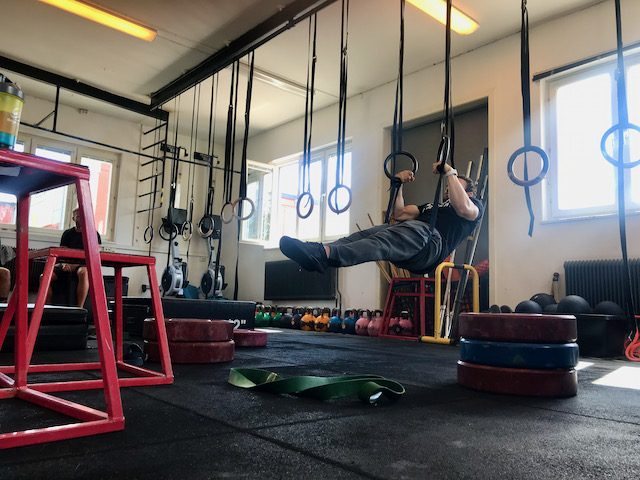
In order to learn a skill, like the strict muscle-up as shown in the video above for example, do we really have to increase the physical training load? Or could we limit explanation and predictions in order to concentrate on when our athletes strugglenow in the skill.
Continuously challenging the individual participant by progressively increasing task difficulty during long-term motor practice enhances motor learning and optimizes performance. Such progressive long-term adaptation to individual skill level not only enhances learning, but does so without necessarily increasing either the volume or the intensity of training.
Simplicity is key both for scalability and to see what is actually driving the trend without the distraction of too many variables. Managing a program of only slight changes and frequent evaluations allows for it to be data driven (as trend analysis is time-sensitive and time-powered).
All of this seems to suggest to use different, not more and often but little-approaches rather than to speculate on theoretical basic capacities, then build a base and to expect linear adaptations.
The old “more is more” approach is still very much ingrained in our way of thinking and planning. That is quite obvious when one looks at and listen to coaches who would subscribe to these theories of learning, but often still feel obliged to offer a progression of physical overload throughout their athletes cycles. Change is quite hard.
Is this the perfect progression to learn or strengthen a skill? Certainly not!
If anything should be clear by now it is that there will always be cases that are different from all other cases. Every method has its place.
I can also picture you thinking that, well, “those examples you have given are too easy. Sure, in strength sports you can get away with performing the specific skill, not something more basic or different, but simply overloaded at the level that the athlete is, but what about other sports not practiced with a barbell or a set of rings?”. Well, stay tuned for more examples of practical implementations of these principles in part 3.
I’ll leave you with the words of the great Touretski, who may have passed on last year, but whose actions and words hopefully will live on for long.
Dare to be different. Doing the same thing as everyone else is a doomed strategy and a flawed philosophy.
“In early life I thought of studying economics, but had found it too difficult!”
Max Planck
In order to optimize performance, training theory has followed it’s fellow scientific endeavors looking deeper and deeper into details of their fields of study in a search for more detailed models of the world. These models are thought to provide more insight into underlying factors of performance. By uncovering them we can then design more meaningful training interventions. This manifests itself in metaphors like “the man as a machine”.
Similar to what Sigmund Freud did in psychology, when he presented the idea that thoughts and emotions outside of our awareness continue to exert an influence on our behavior. Even though we are unconscious of these underlying influences, physiology too has focused on hidden thresholds and reduced causal models of explanation for performance. The hope is to create better and more stable athletes built “from the ground up” and upon more basic conditions for performance than what can be seen with the eye alone.
While this project certainly has merits, it can also obscure the vision from what is “hidden in plain sight”. When searching for what is within and by looking deeper behind what is apparent, you will lose sight of how a scientific area is connected to other scientific areas: how things “just work” in the common world. When one has dug a deep enough hole, he can no longer see over the edge.
Complex biological systems (nature, humans…) are characterized by the fact that they consist of lots of interconnected dependencies in the different parts of its whole. A system constantly exposed to both sensitivity and noise, and a system of constant change.
It’s also quite easy to get stuck in a loop of trying to uncover more and more of these underlying factors, rather than to carry on with whatever knowledge we already have at the moment.
Better than using a detailed map to navigate an ever-changing landscape, like a glacier, would be to routinely triangulate your position and endure living with the degree of inaccuracy and uncertainty that comes with not knowing exactly where you are. Even though the belief in the perfect map gives a sense of security, it is a false feeling that risks leaving us blind to what is actually happening.
Simply observing what we have in front of us is often hard to do.
In order to be able to compare efforts and athletes we usually take the leap from qualitative observation to quantitative data collection, and by doing so removing them further away from the context where they were observed. How do you quantify “fast” or “slow” or “hard” or “easy” without delimiting them by turning them into numbers? Numbers fit so much better in spreadsheets for statistical analysis.
Not only are we by doing so removing the effort out of its context, we are also risking to try to affect these new numbers rather than the situation they emerged in.
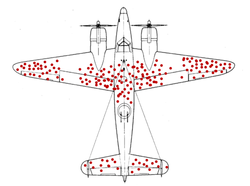
You don’t want your planes to get shot down by enemy fighters, so you armor them. More armor makes a plane heavier and heavier planes are less maneuverable. They also use more fuel. Armoring planes too much is a problem; armoring planes not enough is also a problem.
During the second world war the American army was studying the planes returning from battle and kept reinforcing the areas of the planes that had the highest number of bullet holes. However, more and more planes were lost despite their added protection.
This continued until the statistician Abraham Wald noted that the military only considered the aircraft that had survived their missions. Since they didn’t, or couldn’t, look at the specific battle situations where shots were fired, they failed to see the planes now rendered unavailable from assessment. Wald instead asked: where are there no bullet holes at all?
As aiming at moving planes is not that easy, especially in those times, he figured that the damage would have been spread quite equally all over the plane. Since this did not adhere to the observations, he was fairly sure he knew where the missing bullets were: on the missing planes.
The reason planes were coming back with fewer hits to the engine is that planes that got hit in the engine weren’t coming back. The armor, he said, shouldn’t go where the bullet holes are, but quite the opposite, where the bullet holes aren’t.
At the end they managed to logically figure out a way of protecting their planes. But all of this would have been quite clear if they had not only looked at the data, but also kept an eye on the actual action.
“Mathematics is the source of a wicked intellect that, while making man the lord of the earth, also makes him the slave of the machine.”
Robert Musil
The technology to measure oxygen consumption first arose in the early 1920’s. Using that ability Hill and Lupton found that there appeared to be a maximum limit to oxygen consumption, when despite increases in speed, their VO2 consumption did not also increase any more.
After this most studies in exercise science have been evaluated on the resulting change in VO2max rather than actual performance (such as ability to stay with a breakout, handling of different sections of a race, movement form or even something simple as average speed over a distance). VO2max is less variable and more tolerant to changing conditions. It also happens to fit well into columns of spreadsheets.
As outcomes are increasingly measured by a specific construct, they start to shape the outcomes themselves. Researching training interventions using this or that variable as the standard of success, will slowly shift the training interventions to strengthen just that variable rather than something else. They become self-reinforcing as you will always find more of what you are looking for, and less of what you don’t. Even though that variable might have a very poor transfer on actual sports performance (or health for that matter).
Whenever a new parameter is discovered or introduced, a large degree of emphasis is put on that parameter in the research.
Several new ways of taking measurements of biological processes have had similar impact. With the ability to portably test lactate, research was centered on ways to improve lactate threshold. With the ability to measure force, other variables came into the limelight, such as Functional threshold power or Critical power.
If we all agreed on what math problem we were trying to solve, then we can sit down together and say, hey let’s calculate! But sport and life is messy. We might not agree on what we’re trying to optimize and we also have a lot of uncertainty about what the consequences of our actions will be.
Even with access to great data, not everything’s an optimization problem. Ultimately it is crucial that we understand the limits of the technology we leveraged to help us to navigate our complex world and the values that often invisibly determine how we use it.
“For years we have seen study after study attempting to compartmentalize intensity domains based on an assumption that there is some physiological decompensation point. However we reach no clear consensus on this. First it was MLSS. Then VO2 kinetics. Then FTP and CP, but none are conclusive. Perhaps we are looking for something that isn’t there.”
Dr. Jeroen Swart
We are starting to see why Max Planck, awarded the Nobel Prize, once said that he saw economics as a harder discipline than his own field of theoretical physics: due to the inherent need for subjective judgments. Dealing with humans, is dealing with unpredictability. This could certainly be said about exercise science too.
We often think of these measurable physiological variables as clear cut, defined markers. We use them to train at different thresholds and to classify our training as such. We assume that the transition is clear and that these parameters represent some sort of boundary line, and that improving them leads to better performance.
All of the above mentioned concepts can be helpful, and used to organize and guide training but we need to understand that they do not by themselves represent increased performance. That they do not represent a clearly defined transition. Physiology is complex and messy.
There is no sport of highest VO2max, Critical Power or peak wattage. We should not be so in love with a measurement so that we forget to look at how an athlete handles specific situations of their sports.
”I’ve seen things you people wouldn’t believe. Attack ships on fire off the shoulder of Orion. I watched C-beams glitter in the dark near the Tannhäuser Gate. All those moments will be lost in time, like tears in rain.”
Roy Batty, “Blade Runner”
When you put a pot of liquid water on the stove it is in a steady state. All of the collective molecules exist in liquid form. As soon as you begin applying heat and pressure the state begins to change. At any given point in time we are unable to predict which molecules will make the transition. They exist at the edge of chaos. Provide enough heat and pressure and over time and they will eventually turn into a gas.
Complex systems, such as humans, have interesting properties. Strong interactions between their parts, feedback, emergence, self-organisation, adaptation, growth, change. None of these are a simple linear process. Large interventions in a variable does not necessarily have a large effect on the expected variable of interest. Similarly, a small intervention can have large and unexpected outcomes. Just like a “perfect storm” – a combination of circumstances drastically aggravates the event.
At first this unpredictability is hard to reconcile with. But maybe it’s not necessary to know exactly how a specific performance in such a system emerges?
Continuing with the “perfect storm” analogy, it might be important to provide individuals with periodic interventions that are delivered under varying “atmospheric” (i.e., psychological or life states) conditions. This means providing repeated opportunities to practice this self-organization under realistic conditions.
Consider “Chinese water torture” – a drop of water continuously hitting the same spot on your head for a long time would not bother you at all, but eventually it would change your behavior completely (driving you mad, so don’t use the analogy literally with your athletes).
“We must do away with all explanation, and description alone must take its place [..] The problems are solved, not by giving new information, but by arranging what we have always known“
Ludwig Wittgenstein
Start with what you see. When do athletes struggle in racing or during competition? Describe those situations without explaining why they happen. Separate these situations in the training program and practice them with some variation.
The level of difficulty and overload should not be too high. This might push the system into interpreting the situation as something altogether different from the game-day skill. But not so little that the athlete can complete every repetition with a 100% accuracy (how could a system operating perfectly be pushed into change?).
To practice “what you see the need for” has a few advantages over to base training prescription on hidden underlying qualities
By doing so you will measure its success by exactly the outcome which you want to improve. This prevents you from getting lured in a separate direction by confusing some other variable with performance on the field. Every improvement will have a large transfer from training to performance, making small increases in capacity highly valuable.
You will move into a territory of training which your athletes are familiar with. This helps communication between the two of you. Communication should not be under-valued. When coaches speak the language of science only, how can athletes be expected to understand the drills they are given? You are more likely to get success telling your athlete to “sprint out of that corner as if you would like to get a gap on your opponent” rather than something along the lines of what percentage of VO2 or speed to hit.
It will also help you to get relevant discussions on how to tweak the drills. Although athletes might be lacking in scientific knowledge, they tend to know a fair bit about their sports, and these discussions easily extend into how to use the skills you have been working on when discussing tactics.
The downside is of course that you will have to be open with the fact that all you can offer is educated and well-founded guesses. That there is no magic pill. That all the certainty there is to find is that continually doing the things you wish to improve at over time, with some variance and with some overload is what might increase your capacity (mostly by ways of a sudden phase-transition).
If I could have gotten one dollar every time someone asked me for an assistance exercise for a problem – let’s take the execution of the weightlifting movement of the snatch for instance – and seen the disappointment in their eyes when my first choice of exercise was to do exercises not completely different from with is done in that movement. I’d rather pick an exercise to emphasize or correct the point of the lift where I felt the problematic outcome initially did arise.
This places a lot of demand on the coaches communication skills in order to get the buy-in from the athlete. A buy-in which you could have gotten by dangling a mathematical carrot on a stick in front of the athlete. It will also in my experience bring about more compliance and less injuries when you get the athletes involved in the actual process.
I started working with this young and gifted athlete from Portugal a few years back. He had made the transition from Volleyball into CrossFit where he now had some success, qualifying and performing well at the 2018 Regionals. He also struggled with some of the integral movements of the sport, such as the weightlifting movements – most noticeably the snatch.
He was catching most of his Snatches in front of him, forcing him out of balance. Unfortunately we live at quite some distance and cannot do better than to have close contact over the internet. After a lot of questions and answers and sending videos back and forth we agreed that he had trouble already at the starting position, struggling to find initial balance against the floor. This in turn leads to his position being too upright when the bar passes the knee. His joints then are not properly set up to allow him to hit what in weightlifting is often referred to as thePower position.
Without going into too much detail, the Power position allows for rapid extension of the knee and hip along with plantar flexion, in a sequence called the proximal-to-distal sequence, where extension on the joints one by one allows at least one joint to have a favorable translation relationship throughout the full extension. The failure to hit this position can force the barbells necessary vertical movement slightly forward, getting the lifter into all kinds of problems catching it.
Over the coming period we did quite a lot of
Snatches from power position, with clear instructions on what would constitute a “good rep”, having him to learn and discover on how to generate force from that position. If he could not move from this position without a slight “swinging motion” or if he had to jump forward in the catch he would know that he did not find his Power position properly.
Snatch deadlifts, playing with and learning how balance felt. (Balance is tough, as it is really the absence of feeling. Athletes sometimes tend to seek out more distinctive tension, something they feel, as you would find when you are more on your heels or on your toes)
From knee to power position and from floor to power position.
Full snatches involving the feeling for positions he learned by the above exercises.
Slower, faster… Mixing it up with some fatigue and eventually hitting the positions and moving between them became more second nature for him.
Not once did we do any movement that was fundamentally different from the movement that he struggled with, hoping to increase some “underlying quality” possibly holding him back. Surely, we still trained those underlying qualities, if they existed, by overloading and stressing the movement that involved them. With the added benefit of a more direct transfer and possibly better understanding and feedback of his process.
We also did not measure the performance of the assistance exercises, more than if they successfully challenged the positions where we thought we saw a lack of efficiency and balance. They were always viewed in the light of the performance of the full snatch.
João has gotten more proficient with this movement: here he is, at the end of a 30 minute workout, hitting a 110kg Snatch, rowing 500m in 1 minute and 40 seconds (something not done without breathing hard), then hitting another 110kg snatch just after coming off the rower something that he could not do in isolation before.
Is this the best way to conduct training? Certainly not always! There will always be cases that are different from all other cases. Every method has its place.
It is a simple process helping you not to get completely lost in the “data” jungle, or if you are, to find your way back onto the field, where the actual athletes live.
Stay tuned for more examples of practical implementations of these principles in part 2.
“Science gives direction to the forward movement; while art causes the actual progression. Thus a false activity of science inevitably causes a correspondingly false activity of art.”
Leo Tolstoy
Complementary strength and power training has been shown to be beneficial not only in power sports (throwing, jumping, sprinting, etc) but also in virtually all other sports as well, including team sports (football, rugby, ice hockey etc) and endurance sports (running, cycling, skiing, climbing, etc).
When developing strength training protocols for both team sports and endurance sports the emphasis is rightfully placed upon heavy and/or explosive lifting, because of the inherent potentially high neural drive of this type of training. Bodybuilding type exercises and repetition schemes are stressful on a molecular level, meaning that it might both stimulate undesired hypertrophy and that recovery is long and makes it difficult to combine with sport specific training.
This choice of emphasis often has the effect that coaches do not feel the need to address the exercise selection for their athletes more than to make sure that it provides a high mechanical tension in order to provide a general and abstract high neural drive.
While endurance and team sport athletes are not power sport athletes, and while strength training for them should be treated as general rather than specific, we still should seek to keep exercises somewhat similar in movement patterns and stimuli while providing as large overload as possible. Large loads and heavy weights leads to larger neural adaptation and higher percentage of muscle fibers being recruited, but heavy weights also contribute to change in sensory and intentional qualities and might therefor “unlock” less force production to use in the field of the sport.
When people are overwhelmed by choice and when they are anxious about it, they often turn to denial, ignorance and willful blindness.
Renata Salecl
Often when discussing strength training with endurance or field-sport trainers I am told that “we train deadlifts, because they triggers neural drive”. When I ask if, while being a great exercise, there could possibly be an even better one available for their athletes they usually point to the fact that deadlifts (or whichever other exercise is their catch-all solution) provides neural drive (which implicitly is enough) and that there simply is no need to overthink exercise selection in the weight-room.
With that same reasoning one could advocate to perform only biceps curls, if they would be heavy enough to stimulate increased central motor drive and elevated motoneuron excitability. The response to this is (of course) that, in isolation, “that would not be a great base exercise for cyclists or runners or football players, since it does not involve using the legs”.
My point exactly.
Apparently there are things to consider outside of only the amount of neural drive of an exercise. When taking this too lightly we miss out on the opportunities that might lie buried underneath an attitude of indifference.
In science the expert opinion and the case study is regarded as the lowest type of evidence, as it can only tell you what worked or didn’t work for that one person, in that specific case. In order to say more general things we value science that includes data from more people, as this takes a specific context out of the equation. The more people, the better the prediction of a general average. When such studies also comply to certain standards (randomized and controlled, peer reviewed, published in high impact journals) they represent predictability which is highly regarded in the scientific community.
Systematic reviews and meta-analysis are considered to be the highest-level of evidence available. These types of reports consist of methods for systematically combining study data from several selected studies to develop a single conclusion that has greater statistical power, due to increased numbers of subjects, greater diversity among subjects, or accumulated effects and results.
It would be easy to interpret the results from such studies as the advances toward more and more exact knowledge, when they are in fact the opposite: more broad and general. They are great for predicting the average response in a certain situations, and if you want to be an average coach then you should only base your decisions on studies like these.
But I believe that being a coach should be about trying to beat the average, to be able to provide expert knowledge.
In the real world outside economic theory, every business is successful exactly to the extent that it does something others cannot. Monopoly is therefore not a pathology or an exception. Monopoly is the condition of every successful business.
Peter Thiel
When we accept that our selection of exercises matters, that we can do more than average, we face the risk of being overwhelmed by the sheer abundance of choices we have to make and therefore risk being “paralyzed by analysis”.
Not only that, but we also face the radical uncertainty of the large world: that we do not even know all the possible outcomes. It’s a world that cannot be described in the probabilistic terms of a game of chance because it’s not just that we do not know what will happen, we don’t even know the kinds of things that might happen.
I once read an anecdote about a decision theorist from Columbia University who was struggling whether to accept an offer from a rival university or to stay in his current position. Upon being urged by his colleague to apply his own models of rational decision-making in order to maximize his expected utility he responded with exasperation, “Come on, this is serious”.
To make statements about probability in the real world it is necessary to take into consideration not only the probability derived from the model, but also the probability that the model itself is true. And this we have no way of knowing. We are left to live in a world of unimaginable futures and unpredictable consequences that continue to call for necessary speculation and inevitable disagreement which often never will be resolved.
So when one has lifted ones gaze from the mechanical systems of the average, and now commit to adapt their actions to the situations they have before them, it’s all too easy to be overwhelmed by the sheer amount of options and the impossibility of knowing where the consequences end.
In these cases it seems that we have to remember that the consequences of an action are not everything that follows it forever (any more than the cause of a event is not everything that preceded it). These concepts are made to be used in actual cases where we converse about taking particular actions in our lives. We need to speak about particular circumstances and particular individuals, we need to not only use knowledge about the general (the knowledge we find in systematic reviews and meta-analysis) but also move back to the anecdotal, actual, world.
I do not know – if it matters I will try to find out
Mervyn King, John Kay
It seems we could get some guidelines on how to design complementary training exercises from looking at what principles that apply and what we can say is relevant to the particular situation and person at hand.
if we begin to look at the structure of movement we find that this motor dimension includes characteristics of movement within muscles, between muscles as well as force landscapes and external body posture and joint positions.
Within the muscles there seems to be very little positive transfer between shortening and lengthening of the muscle (concentric and eccentric muscle contractions) and reactivity (using pre-tensioning and energy storage and returning through stiffness). Also, if we are dealing with high intensity sports, the muscle needs to operate at optimal muscle-length and this too limits the possible transfer if training outside of this length when training in the gym (it could actually provide negative transfer if this optimal length is stimulated to change).
When looking at the level of cooperation between muscles the biggest concern should be if our sport carries with it the demand to co-contract in order to be efficient when going from slack to tense. This is usually the case in high speed sports, and if so merely adding load to a movement with the use of barbells or dumbbells should be questioned, simply because of it’s potential to reduce muscle slack as it may not challenge the body to learn to develop proper pre-tension with the use of co-contracting muscles.
Note that adding load likely has benefits, such as forcing the adaption to longer fascicles (able to contract faster than shorter), but we might do well to balance them with ballistic movements from a standstill, and perform some of our heavy lifting from a dead start if this is the case.
There are more ways to waltz, than to sprint
Frans Bosch
In his new book Frans Bosch “Anatomy of agility” discusses, amongst many other things, whether similarity in outward posture is the result of constraints from underlying levels or if it is a separate characteristics of specificity.
He argues strongly that posture is formed out of necessity from the inside rather than that posture shapes the internal movement landscape: given the pressure of time of high intensity movement and the ever-changing environmental influences the body is exposed to, it has to reside to as general principles as possible to be able to adapt. As information from internal force landscapes is more general, it may therefore be more suitable for this than information from posture.
If we look at “what is used in the field”, this is also a strongly rooted approach with expert coaches, who would consider it a bad strategy to first use only soft contacts when striking a boxing bag, hitting a ball or sprinting on the track and only later use forceful technique.
We might do well to no longer proceed our complementary training (or rehabilitation for that matter) from low-intensity to high-intensity, but rather choose to advance from large forces (with few degrees of freedom in movement) to large forces (with increasing degrees of freedom in movement).
Train muscles predominantly similar to the demands of the sport (concentric/eccentric or elastic)
If the demands of the sports is high speed and quick reactions do choose to limit the use of the stretch-shortening reflex.
Do not mimic body positions, mimic force landscapes.
The endurance and field-sport coaches are right when they say that everything we do in the weight-room is by nature unspecific from what their athletes are doing “in the field”. But if we would consider these few points when designing exercises we would likely do better than average. Given that “we do not know what we do not know” I will always advice to do some, but not much, of the things we filter away as well – a smart contingency plan is a staple of good generals.
Do a some very general things as well.
However this is only the physical perspective, we are still dealing with humans. Ask the person in front of you what they consider fun, and make sure to include some of that as well. A program of fantastic and smart exercises, is merely mediocre and stupid if you cannot get anyone to do it.
If someone really enjoy doing something not following from the above list of principles, it is a smart idea to include some of that too.
“O Icarus,” he said, “I warn you: fly a middle course. If you’re too low, sea spray may damp your wings; and if you fly too high, the heat is scorching. Keep to the middle then.
Ovid, “Metamorphoses“
Reading and listening to coaching podcasts these last six months one of the questions that the COVID-19 situation have made people to ask and coaches to ponder is the question of how little one can train in order to not revert the adaptation to training. While one can certainly see why that question would seem important in a world of quarantines and temporary lock-down of training facilities, in many ways it is an expression of the doubtful idea that hidden deep within there is something “naturally you” that you can “enlarge with stress”. A “ground zero” that if not continually challenged you fall back upon.
Hans Selye wrote his famous letter to Nature magazine in 1936, describing how rodents exposed to a variety of nocuous or toxic agents (like cold, surgery, forced exercise, adrenaline and various drugs) responded to these diverse stimulus with pathophysiological changes that had some common features (like enlargement of certain organs). If the treatment was continued with relatively small doses, the animals became resistant and their organs returned to their normal state. Later the terms “general alarm reaction” and “general adaptation syndrome” were proposed for the description of these two phases of the response.
This shaped the current understanding of biological adaptation and the associated terminology, like stress, homeostasis, fight or flight to populate the scientific and popular narrative. A narrative implicating that the physiological stress response follows a stereotypical non-specific trajectory of being predominantly caused by physiological challenge and that its consequences are primarily physiological in nature. Based on this model, for a parameter to deviate from its setpoint value, some internal mechanism must be broken.
In order to force adaptation to training, one should add enough – but not too much – mechanical stress and little by little, in a very predictable way, you would be able to expand your capacity. But as the original setpoint would still be where it always was it would mean that if the stress would discontinue you would fall back to a relatively stable equilibrium maintained by those physiological processes. However evidence accumulates that setpoints are not constant. Their variations, rather than signifying error, are apparently designed to reduce error by anticipating and modulating future needs and resource allocation.
The theory of allostasis proposes that the first mediator – the event first triggering the stress response – is not a physiological stressor. The response is rather triggered by the changing emotional state of the individual brought about by personal interpretation of their capacity to cope with the imposed challenge. This would explain why the structurally rigid and perfectly linear training systems are only successful in text-books, and that we should shift our focus to the increasingly apparent effects of non-physical factors like emotional regulation, anticipation and learning in order to design well functioning training protocols.
In theory there is no difference between theory and practice, while in practice there is
Benjamin Brewster
The perfect predictable plan might be a beautiful idea, but is as likely to be real as the treasure at the end of the rainbow. In reality adaptation is dependent upon context, constitution, history, and persistently transitioning biological states. Studying successful strength-sport coaches will reveal a common theme: very few exercises, relatively consistent loading (even from cycle to cycle) and a focus on technical mastery challenged by increases in perturbations and contextual interferences.
Coaching legend Dan Pfaff, a proponent of minimalist training plans, notes that generally training regiments are too dense and that the goal of a great coach should be to see how little their athletes can do and still improve and be great. It’s all too easy to create an addiction to work and density of work. When new athletes try harder, they get better but there is a tipping point as they develop where this actually becomes a problem, where trying harder no longer works. The athlete is now a different athlete, and would need differentnot more to improve. More will inevitably lead to injury, and injuriesput a stopeverything.
With this in mind the question posed in light of the pandemic seems to be the result of a flawed and potentially dangerous way of thinking. One does not fall back toward anything, as that thing does not exist any more. The exposure to stimulus, both inside and outside of the training facility, constantly changes who you are, not just biologically but also psychologically, and most important of all in a non-linear fashion.
You always adapt into something that is your bodies best guess at what you will be able to cope with in the current and anticipated circumstances. Thinking you do not respond in this way will potentially lead you to fall into the trap of monotony and over-saturation.
And after all, if stupidity did not, when seen from within, look so exactly like talent as to be mistaken for it, and if it could not, when seen from the outside, appear as progress, genius, hope, and improvement, doubtless no one would want to be stupid, and there would be no stupidity.
Robert Musil, “The man with no qualities”
Of course, you would say, but is this really an issue? I mean, you would have seen every coach in the world roll their eyes while talking about other coaches who do not understand this simple point. That “too much is too much” (of course it is) and that “more is not better”. And if everyone is saying that they are not guilty of making these mistakes, then no mistakes are made?
And yes, this might be true, but as true as when you are a little drunk, feeling like a million dollars you tend to fall for the tempting thought that if you double the intake of alcohol you’re gonna have twice the fun! And so, by thinking in linear and physiological terms only, and not considering the effect your (tipsy ?) emotional state has on both stress response and behavior, you go for that quick satisfaction rather than to play the long-game.
And often enough the same coaches use the image of a pyramid when describing how training works, hinting that a stable general base must be built to support the specifics. And is not that an expression of the very same oversimplification as the theory of homeostasis taking on the concept that has been successful when working with things and try to use it when working with humans?
Worse still, backed up with (faulty) logic makes it very hard not to go for the same mistake over and over which I think can be seen in a lot of training programs.
The mental image of the simple and predictable physical universe, where what worked before will always work again is so tempting because it reduces confusion and cognitive dissonance by being inherently measurable. And what is more easily measurable than training volume (but also unfortunately all too easily mistaken for functional productivity)?
I believe in the type of program often referred to as “complex” or “concurrent”. It generally includes no general preparation phases where one would do little to no specificity, as well as no specific preparation phases where one would do the opposite. Instead I have my athletes do a little but not too little of everythingall the time, as growth and self-organization in a dynamic complex system can be the result of an amplification of change elsewhere in the system. Who can tell exactly what an athlete needs to be able to take that next step?
Instead of having the long term macro-perspective control what I do day to day I work with relatively little organizational variation between cycles. Then I monitor how the athletes respond (how they move, how they feel) on a daily or weekly basis. Information I use to prescribe exercises with enough contextual challenge to force adaptation and learning (rather than trying to force this with just more reps). Do I not add workload at all? Sure I do, but I do it based on acute factors rather than from mathematical reasoning.
To provide an insight in how this might look in practice: I usually rotate 2-3 very similar weeks, or blocks if you want to think of it like that. The next rotation does not have changes in loading per se, but novelty is induced by slightly changing how exercises are performed within a fairly general and simple theme.
This example is for our sprint cyclists (who all follow similar outline with some personal adjustments) but I do not structure the complementary training much differently for other cyclists or endurance athletes.
The general idea of force production as a contextual skill is similar for the CrossFit, racket sports or team sports athletes I train, but as their sports are so much more complex (than cycling, running, skiing) the outlines i write for them differ quite a bit. I will follow up with more specific examples of how the training blocks I write for open sports look in a later post.
no wave loading – once a ’program’ is prescribed, it is simply repeated over and over again without much change until an adaptation response is observed – hopefully leading to a phase shift in performance
Some benefits to this type of training is that it makes it easy to adapt to with actual performance goals in mind. Programs that empathize large variations in between phases will make it hard to see what is actually driving the trend. The smaller, simpler program allow for scalability and for data collection of the most important variables all season long.
Other benefits are that one constantly addresses the systems long-term behavior, producing a stable state of performance. While one might not always be on the absolute top, we’re always damn close to it without any drastic changes either in volume or intensity. By doing so we are reducing the risk of injury from either over or under-training.
Got to hurry, got to hurry, I don’t believe you worry Take it back, take it back, You know you can’t do that Don’t want no sleep, Just hide and seek Yes, I’m a speedfreak, Baby, I’m a speedfreak
Motorhead
As sprinters we want to be able to move our feet as fast as possible. Regardless if we are clicked into pedals on a bike, wearing spikes running down a track or on the field in a team sport we do want to get our speed of movement as high as possible for our activity. But we are not thrown out of an airplane, finding ourselves moving as fast as we possible can with no effort. We need to get up to speed all by ourselves, by accelerating our body.
With every step or every revolution of the pedal, if our power is higher than the braking forces acting upon us our speed of movement increases, until at some point the net forward momentum equal to those braking forces and we are now moving at maximum velocity.
In track and field events extending the acceleration phase is something positive and largely correlated with lower sprinting times and better chance of winning. This comes from the fact that if you can push your acceleration phase from 25m (normal for a beginner) to 70m (world record 100m runner) then your speed at the end of that acceleration is higher, but also, since that maximum speed cannot be maintained for a very long time, that the deceleration phase of the race will be shorter. Even a short race like the 100 meters is damn long if there is 70m to go when you’re entering the “die a glorious death”-phase (or, if you’re unlucky, just the “die a death”-phase).
Actually, when it has been modeled, a longer acceleration phase always wins over a shorter one and thus the objective for a 100m sprinter should always be to increase the maximal speed, as this will also emphasize to keep accelerating. For as long as the race is if that was possible.
For the team sport athlete, or the cyclist, there are however other things to consider. The dream scenario of the straight sprint down the full fields in football or rugby, is never more than just a dream as the opponents are eager to crush you with a tackle. This makes the rate of acceleration even more important as you want to be able to get up to speed and past that defender in the little time and distance available.
One would think situation for the cyclist would be similar to the 100m runner, but there are several differences that motivates him or her, similarly to the field sport athlete, to increase the rate of acceleration rather than to extend the distance of it.
While the braking force of air resistance for the runner is not something that he or she can affect much – it is what it is – this is not true for the cyclist but something that can be changed to a large degree by assuming more aerodynamic posture on the bike. While the biomechanical characteristics of the standing position offers the higher power outputs suitable for creating the high forces needed to accelerate, the seated position offers kinematic, energy cost and mechanical efficiency.
Aerodynamic drag is by far the most significant variable for cycling, increasing by the square of our speed until accounting for 90% of total resistance over 50kph. The cyclist will at some point be able to increase his speed more by sitting down forming a smaller frontal area rather to try to extend the standing acceleration phase. Because of this the cyclist benefit from accelerating quickly in order to reap the advantages available by “going low” earlier than his opponents, spending less energy while preserving his or her speed.
If we consider track cycling there are even more constraints, as we also will not be able to keep standing up when going fast. The speed will increase the G-forces in the curves which will eventually push us down into the saddle. This makes most track cyclists stand up only until riding into the second curve (turn 3 or 4 if you talk “track geography”), giving them a distance to accelerate of something between 150 and 200m, depending on how strong and fast they are and what gearing they ride.
Speed, it seems to me, provides the one genuinely modern pleasure.
Aldous Huxley
So there is a difference between how to approach complementary training of maximal speed in track and field versus in field sports and cycle sprinting. In the former you could anchor the training prescription from the speed side, as it should also carry over to the improved acceleration necessary to reach higher speed, but in the latter ones we probably should address the training from more of an emphasis on acceleration. Limited by time or distance we likely should seek to improve the rate of acceleration, always get stronger and more powerful.
While there is a lot to gain at high stride or pedaling frequencies from increased tendon stiffness, when it comes to increase the rate of acceleration at lower velocities we would likely need to produce more muscular force down into the pedals or ground, something ordinarily categorized as increased strength.
Similar to the acceleration phase in track and field there is an change in the relative contribution of horizontal (forward motion of the hip) and vertical application of force in cycling. In the track and field this relative horizontal movement is largest when exiting the starting blocks until at maximal velocity almost all force is directed straight down into the ground. When out of the saddle in cycling, as speed and cadence is increased, horizontal movement of the hip also is reduced until it is more or less locked over the saddle. So when selecting exercises to provide overload to support the acceleration phase it seems reasonable to have some orientation of the force forward.
During a sprint the max power is reached within the very first seconds of the effort, but does not last long because the optimal loading conditions for power are changed with the increase of speed. With so little stimulus at this optimal velocity for power per interval of training it makes for many hard efforts to provide enough “hits at the system” to force adaptation.
Like I highlighted when describing a process for selecting complementary exercises for the start in my last article, we should seek to find exercises that provide some similarity of sensory patterns and intention. This should enhance the possibility of transferring the strength from the gym to the field of the sport. This though process should make us give prominence to exercises that has a somewhat similar finishing position as in the sport. It would also be a bonus if the starting position is distinct and if there is some actual movement of the body in the direction that the sport.
Pictures borrowed from Dan McPartlans prestentation “Why are ankles important to cycling”, see article notes.
Pedal force is ultimately produced by the muscles that span the hip, knee and ankle joints. The main function of the hip extensors and knee extensors is to generate force that is to be transferred to the pedal. It has been shown that exercises where the muscle is shortening (concentric) and exercises where the muscle is lengthening (eccentric) both are able to increase the muscles ability to forcefully open these joints.
However, as discussed in the previous article, there are some possible downside with pre-loading with a counter-movement or a slow eccentric action as it might impair the body ability to use co-contractions. Co-contractions are the only efficient option available “on the field” to reduce the muscle-slack that has to be taken care of before being able to produce movement, and this ability should be safeguarded.
The calf muscles have two functions: in addition to producing pedal force themselves they must also stiffen the ankle so that the force developed by the knee and the hip can be effectively transferred to the pedal. If your ankle-foot system is not able to transmit that force, “deforming” under tension, this impairs your technique and by extension radically impairs your performance. This stiffening of the ankle also has to happen really quickly in order for as little as possible of such leakage of force to occur.
The maximum force developed by a muscle is proportional to the number of sarcomeres, the basic contractile unit of muscle fiber, in parallel while the maximum shortening velocity is proportional to the number of sarcomeres in series.
With their pennate structure, allowing for more sarcomeres in parallel, the calf muscles are perfect for very brief efforts of very high force production. In order to support this they are also designed for a “pumping” or recurring function such as in running and cycling. In longer duration actions the blood circulation needed for this is impaired, as exposed by the sensation of pain (“the pump”) that accompanies such exercises (for example the calf raise).
Because of it’s muscle fiber orientation the calf muscles are not really suited for generating a large range of motion, and when they are used in sports remains more or less the same range (isometric). This optimum length of tension in muscle can be shifted to longer muscle lengths, especially by large range of motion eccentric exercise, but altering this length-tension relationship in a muscle could also alter it’s function and might be something to avoid for muscles of this type.
Let’s reiterate.
When selecting complementary exercises for the acceleration phase (out of the saddle) of cycle sprinting we would like to find exercises that
Extend the time at high power production, at what we can call “optimal velocity”, in order to get “stronger” and be able to accelerate faster.
Limit the possible pre-stretch or slow eccentric action that could affect the co-contraction ability that is necessary for the muscles to be efficient at going from slack to tense.
Work the muscles around the hip and knee joints mainly through shortening (concentric action) while at the same time work the calf and ankles mainly at constant length (isometric action).
Provide muscular overload and if possible, provide sensory similarity in body positioning and movement.
Sprinting on a slight incline is a good way of adding resistance and by doing that also maintain the athlete at conditions around maximum power. However doing this in the gym, where higher overload than in the specific conditions that is to be found on the bike could and should be sought, is more complicated. One could try to use a air and magnet resisted devices like the Wattbike, but while providing both a resistance increasing both exponentially and linearly with speed, it fails to provide the high force demands found in the inertia of the initial acceleration. While coming close, it just does not feel the same at those first few seconds.
When adding load to a sled and pushing or pulling it, we also, in addition to the increased resistance of the mass being accelerated (bodyweight plus sled) have to fight friction. While this coefficient of resistance will vary with different sleds (new, old, rusty?) and different surfaces (dry asphalt, wet turf?) it will always provide resistance to prolong conditions similar to the “optimal velocity” in the beginning of the acceleration, and provide more “stimuli per set” than unloaded acceleration.
The overload generated by heavy sleds should add to lower limb strength, and possibly also help to transfer strength from other less contextual strength movements like the squat into cycling (or running). This overload is placed upon all the joints simultaneously, including the often forgotten ankle joint. The sled push is also working the hip and knee joints with concentric action, while the ankle joint works isometrically, supporting their respective functions in forward acceleration.
While the definite answer to if one should load the sleds heavy or light is not yet established, there are vast amount of data suggesting to go heavy rather than not. The eminent French scientist JB Morin notes that without heavy loads, mechanical exposure to very acute angles is not possible compared to when using light loads.
Considering that we established that the sprint cyclist would rather seem to prefer increased muscular strength over tendon stiffness in order to increase the rate of acceleration, and if we accept that more overload likely shifts the adaptation in this direction then it seems reasonable to go for heavy loads.
I would make three arguments for deciding to push the sled, rather to pull it forward. First, the pushing style seem to make athletes to be able to work with heavier weights, which might be able to shift the adaptation to our muscular preference. Second, pushing with the arms does appear to further increase forward lean and alter foot placement, which may favor increased horizontal impulse. Third and possibly most important, having tension throughout the whole body, from the hands to the feet pushing into the ground is more contextual than having the hands free. The longer chain of activation is, even though in cycling we pull ourselves down rather than push our way forward, likely to be more similar in intermuscular demands of transferring force through joints all the way down to the feet.
How heavy is heavy? Well, rather than trying to find the optimal individual load it has been shown that to use a percentage of body weight correlates well between individual load and performance. In studies the groups using “very heavy” loads has been using ~80% of their body weight on the sled, but since this has been pulled rather than pushed I would not hesitate to go heavier.
In our never ending pursuit to ride bigger gears, maybe we should also strive to always push heavier sleds?
“The first step towards getting somewhere is to decide that you are not going to stay where you are.“
J.P. Morgan
The posterior chain is primarily composed of four muscle groups: the calves, the hamstrings, the glutes and the spinal erectors.
The benefits of strengthening the posterior chain in cyclists is not as well established in cycling as in running, but there is no reason to doubt that they are significant. We want to avoid injuries of the like of that hamstring strain that kept four time Olympic gold medalist Laura Kenny on the sidelines in 2017. Secondly, the posterior chain seems to be a substantial contributor to performance.
Hamstring injuries are usually caused by a moment of rapid acceleration, deceleration or intense physical effort and while all too common in running, football, rugby and athletics unfortunately we do experience them in the sport of cycling as well. Knowing of the increased exposure to risk of injury when applying high power to the pedals, it should come to no surprise that they are common in the sprint oriented disciplines. Because of changed behavior between and within muscles when exposed to fatigue, that too could be the cause of a “pulled hamstring”.
While the amount of injuries of the posterior chain in cycling are not to be taken lightly, they are less common than in sports where you absorb higher forces from the ground. This makes performance the more important reason for training the muscles of the posterior chain for cyclists.
When the relationship between the exercise performance and lower limb muscle fatigue in cycling has been explored it has been shown that the two muscles most closely correlated with producing and sustaining high power are the Vastus Lateralis and the Hamstrings. Vastus Lateralis of course, the big muscle of the front legs, would be the usual guess but the significant role of the Hamstrings to the influence of exercise performance might come as a surprise.
Maximum force development takes time, and because time is limited in cycling as in almost all sports, the capability to rapidly develop force is crucial to maximize performance. When we pedal we need to be able to generate as much force as possible, as quickly as possible, before the pushing leg must relax in order to not act against the push of our other leg. Also, both for performance and for injury prevention, we should be as fatigue resistant as possible in order to turn around our pedals as efficiently as possible
The use of Hip thrust, Leg curl, Nordic curl, Deadlift – or the nowadays more popular Romanian deadlift – and Kettlebell swings are commonly used in the gym to train the posterior chain, and while all of these exercises do train the right muscles and do have merits I believe there are even better ones available.
“If risks are known, good decisions require logic and statistical thinking. If some risks are unknown, good decisions also require intuition and smart rules of thumb”
Gerd Gigerenzer
The strategy of embracing uncertainty, to deploy an intermittent decision process rather than to make that grandiose plan that could only work in a fixed and predictable world would tell us to give up finding the perfect solution. One should probably do a little of everything, all the time, as growth and self-organization in an dynamical complex system can be the result of an amplification of change elsewhere in the system. However, as we simply cannot do this, do everything, we still need to decide upon where to start.
So, let’s reiterate the list of criterion for strength work in the gym that we settled on in the Strong legs makes their own path articles, in order to see if we could use those criterions to help us in our decision process.
Keep movement somewhat similar in movement patterns and stimuli
Overload as much as possible while satisfying the first rule. Large load means larger neural adaptation and higher percentage of muscle fibers being recruited.
When we are keeping volumes lower and intensity higher, we get what we need from a strength point of view while avoiding being overly tired from too much complementary training. Something that could render us unable to do well on the field where that important true specificity is to be found. If we’d like to keep volume low we’d be smart to stick to few, but efficient exercises.
We could get some help to discard the exercises that are not efficient enough by examining academic studies that has been researching the muscle level activation performed with different exercises. From doing that we seem to learn to favor the Romanian deadlift and the Glute ham raise/Nordic curl rather than the leg curl and good morning.
We have more to consider! To assist the rate of force development and fatigue resistance, I would like to add the following to the list of criterion:
We should prefer exercises that increase our ability to generate force, quickly, and should avoid exercises that negatively impact this capability
Seek to improve strength endurance sufficiently in order to sustain power and decrease the risk of injury
“Faster, Faster, until the thrill of speed overcomes the fear of death.”
Hunter S. Thompson
When a muscle is not activated, it is relaxed. There is slack in both the muscle and tendon. Before they can generate movement of the body it first has to take up the slack and go “tense”. Some athletes struggle to produce this tension and removal of slack quickly (early phase rate of force development) and it can hinder their performance.
In many athletic movements, such as sprints, changes of direction, throws, kicks, etc, the time which force can be generated against the ground or an object is lower than 250 milliseconds. If we are inefficient at going from slack to tense this can take up to 100 milliseconds of that time without even accomplishing movement, something that could severely hindering performance. This is also likely the case in cycling, where the optimal pedaling rate for high power sprinting seems to be somewhere around 120 revolutions per minute. 120 rpm’s means 500 milliseconds per cycle, where about half of that is comprised of leg extension and the rest needed to finalize relaxation in order to let the other leg take its turn.
Strategies to reduce muscle slack is to create pretension using co-contractions, using counter movements or by adding load. This is, for instance, why a rebounding “counter movement jump” is always higher than a “squat jump” starting from a static bottom position. Better results in training can be deceiving, as practicing counter movements leads to decreased ability to produce co-contractions without the counter movement (which most sport lack time to perform on the field, and which does not exist in cycling).
Observe that claims of adding load to a movement with the use of barbells or dumbbells should be questioned, simply because of it’s potential to reduce muscle slack as it may not challenge the body to learn to develop proper pre-tension with the use of co-contracting muscles.
There are other benefits of high overload of course, but it is important to search for a balance between the possible negative effects on pre-tensioning abilities and the positive effects force production. This balance may well be carried out by emphasizing movements from a “dead” start rather than with an eccentric movement. Seemingly this could make us prefer, for instance, the regular Deadlift over the Romanian deadlifts and the Nordic raise.
For the high power ballistics movements such as jumps and throws this means to include variations, possible more often than not, from static positions even though it likely means less impressive results in the training hall.
Force production is linked to related movement patterns, not only in similar physical structure but also in similarity of sensory patterns (seeing and feeling) and intention. This means that we should, if we can, try to get some similarity of the end, and if possible, start positions when overloading a sport specific movement in the gym.
I would argue that all barbell versions of the Deadlift as well as the Nordic curl, despite highly activating the right muscles, lack in this area for all movements performed on a bike regardless if it’s in or out of the saddle. I would probably argue the same for most other sports as well, and I would want to propose the Death march as an alternative that should be strongly considered.
Regardless of being performed by “from the top”, lowering the weights, it has a finishing position similar to both cycling and running, and when used with a dead start it also has a similar start position. Adding to this is that it, similar to most sports, offers actual forward movement rather than standing still. This could very well offer better transfer into the field of play while still be possible to overload with quite large loads.
When it comes to injury prevention to fatigue resistance the slow negative provided by the Romanian deadlift or the Nordic curl are both viable solutions, but as we recognized, possibly with a cost when it comes to explosiveness.
It has been proposed by the same dutch scientists that popularized the concept of muscle slack, Bas Van Hooren and Frans Bosch, that contraction intensity may be the main stimulus for improvements seen with negative training and that isometric training – when the muscle doesn’t noticeably change length and the affected joint doesn’t move – could therefore also be highly effective when performed at a high contraction intensity.
Further, isometric exercises permits us to control at which muscle-length they are performed, opening up the potential for them to be performed at a sport specific length or around the optimum length where higher forces than a lowering only exercise can produce. This could allow for more adaptation with less overall volume, leaving more energy to hit the sport specific work.
Van Hooren proposes integrating progressively harder single leg holds, around 10 seconds of work performed for three sets, going from bodyweight only into slightly weighted into upper body rows and I have used this progression successfully.
Dealing with the radical uncertainty of biological systems it is probably wise to hedge our bets with multiple types of exercises, as we do not know what will be pushing the system into that state of increased performance and injury sustainability. Therefore, for athletes with two days of strength training per week I tend to program the Death march and the isometric holds on one of those, and to do a Deadlift variation and Nordic curls for the other session.
“Pedaling Performance Changing of Elite Cyclists Is Mainly Determined by the Fatigue of Hamstring and Vastus Muscles during Repeated Sprint Cycling Exercise”, https://www.hindawi.com/journals/bmri/2020/7294820/